• Ordinary Differential Equations
  • What Is An ODE
    • Exact Solutions
    • Linear Systems
  • Solving An ODE Numerically
  • Owl-ODE
    • Example: Linear Oscillator System
    • Solver Structure
    • Symplectic Solvers
    • Features and Limits
  • Examples of using Owl-ODE
    • Explicit ODE
    • Two Body Problem
    • Lorenz Attractor
    • Damped Oscillation
  • Stiffness
    • Solve Non-Stiff ODEs
    • Solve Stiff ODEs
  • Summary

« Back to homepage

Ordinary Differential Equations

A differential equation is an equation that contains a function and one or more of its derivatives. It is studied ever since the invention of calculus, driven by the applications in mechanics, astronomy, and geometry. Currently it has become an important branch of mathematics study and its application is widely extended to biology, engineering, economics, and much more fields. In a differential equation, if the function and its derivatives are about only one variable, we call it an Ordinary Differential Equation (ODE). It is often used to model one-dimensional dynamical systems. Otherwise it is an Partial Differential Equation (PDE). In this chapter we focus on the ODE and introduce what is it, how it can be solved numerically, and the tools we provide to do that in Owl.

What Is An ODE

Generally, an ODE can be expressed as:

\(F(x, y^{'}, y^{''}, \ldots, y^{(n)}) = 0.\)

The differential equations model dynamic systems, and the initial status of the system is often known. That is called initial values. They can be represented as:

\[y|_{x=x_0} = y_0, y^{'}|_{x=x_1} = y_1, \ldots\]

where the \(y_0\), \(y_1\), etc. are known. The highest order of derivatives is the order of this differential equation. A first-order differential equation can be generally expressed as: \(\frac{dy}{dx}=f(x,y)\), where \(f\) is any function that contains \(x\) and \(y\). Solving the equation that fits the given initial values is called the initial value problem. Solving problems of this kind is the main target of many numerical ODE solvers.

Exact Solutions

Solving a differential equation is often complex, but we do know how to solve part of them. Before looking at the computer solvers to a random ODEs, let’s turn to the math first and look at some ODE forms that we already have analytical close-form solution to.

ODE	Solution
\(P(y)\frac{dy}{dx} + Q(x) = 0\)	\(\int^{y}P(y)dy + \int^{x}Q(x)dx = C\)
\(\frac{dy}{dx} + P(x)y = Q(x)\)	\(y=e^{-\sum_{x_0}^xP(x)dx}(y_0 + \sum_{x_0}^xQ(x)e^{\sum_{x_0}^xP(x)dx}dx)\)

The table shows two examples. The first line is a type of ODEs that are called the “separable equations”. The second line represents the ODEs that are called the “linear first-order equations”. The solutions to both form of ODE are already well-known, as shown in the second column. Here \(C\) is a constant decided by initial condition \(x_0\) and \(y_0\). \(P(x)\) and \(Q(x)\) are functions that contain only variable \(x\). Note that in both types the derivative \(dy/dx\) can be expressed explicitly as a function of \(x\) and \(y\), and therefore is called explicit ODE. Otherwise it is called an implicit ODE.

High order ODEs can be reduced to the first order ones that contains only \(y'\), \(y\), and \(x\). For example, an ODE in the form \(y^{(n)} = f(x)\) can be reduced by multiple integrations one both sizes. If a two-order ODE is in the form \(y^{''} = f(x, y')\), let \(y' = g(x)\), and then \(y^{''} = p'(x)\). Put them into the original ODE, and it can be transformed as: \(p'=f(x,p)\). This is a first-order ODE that can be solved by normal solutions. Suppose we get \(y'=p=h(x, C_0)\); this explicit form of ODE can be integrated to get: \(y = \int~h(x, C_0)dx + C_1\).

We have only scratched the surface of the ODE as traditional mathematics topic. This chapter does not aim to fully introduce how to solve ODEs analytically or simplify high-order ODEs. Please refer to classical calculus books or courses for more detail.

Linear Systems

ODEs are often used to describe various dynamic systems. In the previous examples there is only one function y that changes over time. However, a real world system often contains multiple interdependent components, and each can be described by a unique function that evolves over time. In the next of this chapter, we will talk about several ODE examples in detail, such as the two-body problem and the Lorenz attractor. For now, it suffices for us to look at equations in the sections below and see how they are different from the single-variant ODE so far. For example, the Lorenz attractor system has three components that change with time: the rate of convection in the atmospheric flow, the horizontal and vertical temperature variation.

These two systems are examples of what is called the first-order linear system of ODE or just the linear system of ODE. Generally, if we have:

\[\boldsymbol{y}(t) = \left[\begin{matrix}y_1(t) \\ \vdots \\ y_n(t) \end{matrix} \right], \boldsymbol{A}(t) = \left[\begin{matrix}a_{11}(t) & \ldots & a_{1n}(t) \\ \vdots & \ldots & \vdots \\ a_{n1}(t) & \ldots & a_{nn}(t) \end{matrix} \right], \textrm{and } \boldsymbol{g}(t) = \left[\begin{matrix}g_1(t) \\ \vdots \\ g_n(t) \end{matrix} \right],\]

then a linear system can be expressed as:

\[\boldsymbol{y'}(t) = \boldsymbol{A}(t)\boldsymbol{y}(t) + \boldsymbol{g}(t).\]

This linear system contains \(n\) time-dependent components: \(y_1(t), y_2(t), \ldots, y_n(t)\). As we will be shown soon, the first-order linear system is especially suitable for the numerical ODE solver to solve. Therefore, transforming a high-order single-component ODE into a linear system is sometimes necessary, as we will show in the two body problem example. But before we stride too far away, let’s get back to the ground and start with the basics of solving an ODE numerically.

Solving An ODE Numerically

This section introduces the basic idea of solving the initial value problem numerically. Let’s start with an example:

\[y' = 2xy + x,\]

where the initial value is \(y(0) = 0\). Without going deep into the whole math calculation process (hint: it’s a separable first-order ODE), we give its analytical close-form solution:

\[y = 0.5(e^{x^2} - 1).\]

Now, pretending we don’t know the solution, we want to answer the question: what is \(y\)’s value when \(x = 1\) (or any other value)? How can we solve it numerically?

Enter the Euler Method, a first-order numerical procedure to solve initial value problems. The basic idea is simple: according to the equation, we know the derivative, i.e., the “slope” at any given point on the function curve. Besides, we also know the initial value \(x_0\) and \(y_0\) of this function. We can then simply move from the initial point to the target \(x\) value in small steps, and at every new point we adjust the direction according to derivative. Formally, the Euler method proposes to approximate the function \(y\) using a sequence of iterative steps:

\[y_{n+1} = y_n + \Delta~f(x_n, y_n),\]

where \(\Delta\) is a certain step size. This method is really easy to be implemented in OCaml, as shown below.

let x = ref 0.
let y = ref 0.
let target = 1.
let step = 0.001
let f x y = 2. *. x *. y +. x

let _ =
  while !x <= target do
	y := !y +. step *. (f !x !y);
	x := !x +. step
  done

In this case, we know that the analytical solution at \(x=1\) is \(0.5(e^{1^2} - 1)\):

# (Owl_const.e -. 1.)/. 2.
- : float = 0.859140914229522545

and the solution given by the previous numerical code is about 0.8591862, which is pretty close to the true answer.

However, this method is as easy as it is unsuitable to be used in practical applications. One reason is that this method is not very accurate, despite that it works well in our example here. We will show this point soon. Also, it is not very stable, nor does it provide error estimate. Therefore, we can modify the Euler’s method to use a “midpoint” in stepping, hoping to curb the error in the update process:

\[s_1 = f(x_n, y_n),\] \[s_2 = f(x_n + \Delta~/2, y_n + s_1~\Delta~/2),\] \[y_{n+1} = y_n + \Delta~\frac{s_1 + s_2}{2}.\]

This method is called the Midpoint Method, and we can also implement it in OCaml similarly. Let’s compare the performance of Euler and Midpoint in approximating the true result:

let f x y = 2. *. x *. y +. x
let f' x = 0.5 *. (Maths.exp (x *. x) -. 1.)

let euler step target =
	let x = ref 0. in
	let y = ref 0. in
	while !x <= target do
		y := !y +. step *. (f !x !y);
		x := !x +. step
	done;
	!y

let midpoint step target =
	let x = ref 0. in
	let y = ref 0. in
	while !x <= target do
		let s1 = f !x !y in
		let s2 = f (!x +. step /. 2.) (!y +. step /. 2. *. s1) in
		y := !y +. step *. (s1 +. s2) /. 2.;
		x := !x +. step
	done;
	!y

let _ =
	let target = 2.6 in
	let h = Plot.create "plot_rk01.png" in
	Plot.(plot_fun ~h ~spec:[ RGB (66,133,244); LineStyle 1; LineWidth 2.; Marker "*" ] f' 2. target);
	Plot.(plot_fun ~h ~spec:[ RGB (219,68,55); LineStyle 2; LineWidth 2.; Marker "+" ] (euler 0.01) 2. target);
	Plot.(plot_fun ~h ~spec:[ RGB (219,68,55); LineStyle 2; LineWidth 2.; Marker "." ] (euler 0.001) 2. target);
	Plot.(plot_fun ~h ~spec:[ RGB (244,180,0); LineStyle 3; LineWidth 2.; Marker "+" ] (midpoint 0.01) 2. target);
	Plot.(plot_fun ~h ~spec:[ RGB (244,180,0); LineStyle 3; LineWidth 2.; Marker "." ] (midpoint 0.001) 2. target);
	Plot.(legend_on h ~position:NorthWest [|"Close-Form Solution"; "Euler (step = 0.01)";
		"Euler (step = 0.001)"; "Midpoint (step = 0.01)"; "Midpoint (step = 0.001)"|]);
	Plot.output h

Let’s see the result.

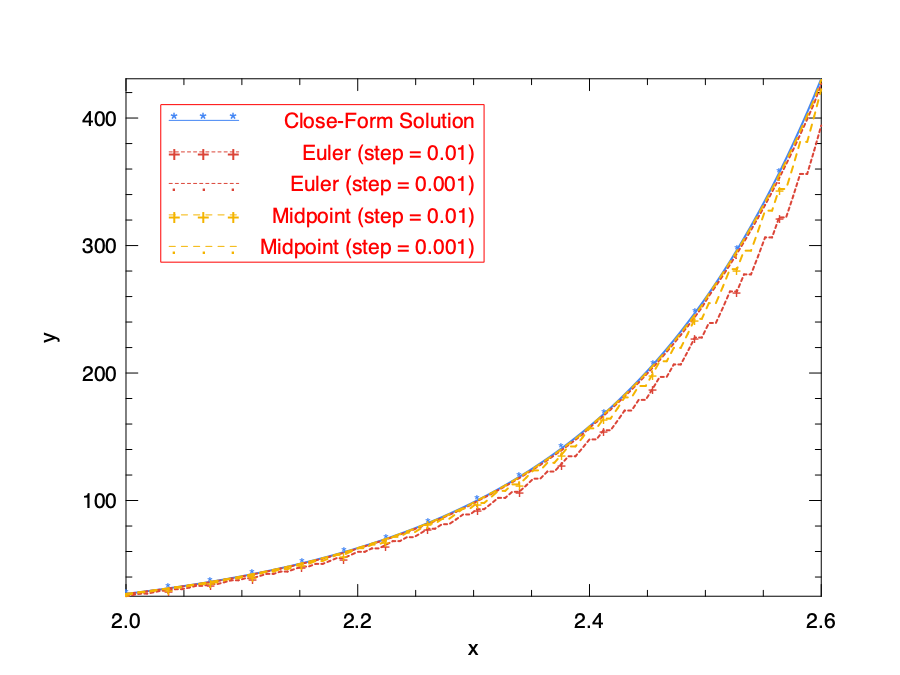
We can see that the choice of step size indeed matters to the precision. We use 0.01 and 0.001 for step size in the test, and for both cases the midpoint method outperforms the simple Euler method.

Should we stop now? Do we find a perfect solution in midpoint method? Surely no. We can follow the existing trend and add more intermediate stages in the update sequence. For example, we can do this:

\[s_1 = f(x_n, y_n),\] \[s_2 = f(x_n + \Delta~/2, y_n + s_1~\Delta~/2),\] \[s_3 = f(x_n + \Delta~/2, y_n + s_2~\Delta~/2),\] \[s_4 = f(x_n + \Delta, y_n + s_3~\Delta),\] \[y_{n+1} = y_n + \Delta~\frac{s_1 + 2s_2+2s_3+s_4}{6}.\]

Here in each iteration four intermediate steps are computed: once at the initial point, once at the end, and twice at the midpoints. This method is often more accurate than the midpoint method.

We can keep going on like this, but hopefully you have seen the pattern so far. These seemingly mystical parameters are related to the term in Taylor series expansions. In the previous methods, e.g. Euler method, every time you update \(y_n\) to \(y_{n+1}\), an error is introduced into the approximation. The order of a method is the exponent of the smallest power of \(\Delta\) that cannot be matched. All these methods are called Runge-Kutta Methods. The basic idea is to remove the errors order by order, using the correct set of coefficients. A higher order of error indicates smaller error.

The Euler is the most basic form of Runge-Kutta (RK) method, and the Midpoint is also called the second-order Runge-Kutta Method (rk2). What the equation shows is a fourth-order Runge-Kutta method (rk4). It is the most frequently used RK method and works surprisingly well in many cases, and it is often a good choice especially when computing \(f\) is not expensive.

However, as powerful as it may be, the classical rk4 is still a native implementation. A modern ODE solver, though largely follows the same idea, adds more “ingredients”. For example, the step size should be adaptively updated instead of being constant as in our example. Also, you may have seen solvers with names such as ode45 in MATLAB, and in their implementation, it means that this solver gets its error estimate at each step by comparing the 4th order solution and 5th order solution and then decides the direction.

Besides, other methods also exist. For example, the Adams-Bashforth Method and Backward Differentiation Formula (BDF) are both multi-step methods that utilise not just the information such as derivative of the current step, but also of previous time steps to compute the solution at next step. In recent years, the Bulirsch-Stoer method is known to be both accurate and efficient computation-wise. Discussion of these advanced numerical methods and techniques are beyond the scope of this book.

Owl-ODE

Obviously, we cannot just rely on these manual solutions every time in practical use. It’s time to use some tools. Based on the computation functionalities and ndarray data structures in Owl, we provide the package “owl_ode” to perform the tasks of solving the initial value problems. Let’s start by seeing how the owl-ode package can be used to solve ODE problems.

Example: Linear Oscillator System

Here is a time independent linear dynamic system that contains two states:

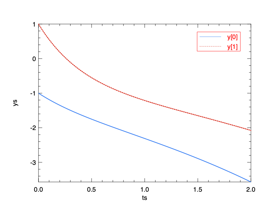
\[\frac{dy}{dt} = Ay, \textrm{where } A = \left[ \begin{matrix} 1 & -1 \\ 2 & -3 \end{matrix} \right].\]

This equation represents an oscillator system. In this system, \(y\) is the state of the system, and \(t\) is time. The initial state at \(t=0\) is \(y_0 = \left[ -1, 1\right]^T\). Now we want to know the system state at \(t=2\). The function can be expressed in Owl using the matrix module.

let f y t =
  let a = [|[|1.; -1.|];[|2.; -3.|]|]|> Mat.of_arrays in
  Mat.(a *@ y)

Next, we want to specify the timespan of this problem: from 0 to 2, at a step of 0.001.

let tspec = Owl_ode.Types.(T1 {t0 = 0.; duration = 2.; dt=1E-3})

One last thing to solve the problem is the initial values:

let x0 = Mat.of_array [|-1.; 1.|] 2 1

And finally we can provide all these information to the rk4 solver in Owl_ode and get the answer:

# let ts, ys = Owl_ode.Ode.odeint Owl_ode.Native.D.rk4 f x0 tspec ()
val ts : Owl_dense_matrix_d.mat =

   C0    C1    C2    C3    C4     C1996 C1997 C1998 C1999 C2000
R0  0 0.001 0.002 0.003 0.004 ... 1.996 1.997 1.998 1.999     2

val ys : Owl_dense_matrix_d.mat =

   C0       C1       C2       C3       C4        C1996    C1997    C1998    C1999    C2000
R0 -1   -1.002 -1.00399 -1.00599 -1.00798 ... -3.56302 -3.56451   -3.566 -3.56749 -3.56898
R1  1 0.995005 0.990022 0.985049 0.980088 ... -2.07436 -2.07527 -2.07617 -2.07707 -2.07798

The rk4 solver is short for “forth-order Runge-Kutta Method” that we have introduced before. The result shows both the steps \(ts\) and the system values at each step \(ys\). We can visualise the oscillation according to the result:

Solver Structure

Hope that you have gotten the gist of how to use Owl-ode. From these examples, we can see that the owl-ode abstracts the initial value problems as four different parts:

1. a function \(f\) to show how the system evolves in equation \(y'(t) = f(y, t)\);
2. a specification of the timespan;
3. system initial values;
4. and most importantly, a solver.

If you look at the signature of a solver:

val rk4 : (module Types.Solver
    with type state = M.arr
    and type f = M.arr -> float -> M.arr
    and type step_output = M.arr * float
    and type solve_output = M.arr * M.arr)

it clearly indicates these different parts. Based on this uniform abstraction, you can choose a suitable solver and use it to solve many complex and practical ODE problems. Note that due to the difference of solvers, the requirement of different solver varies. Some requires the state to be two matrices, while others process data in a more general ndarray format.

Owl-ode provides a wide range of solvers. It implements native solvers which are based on the step-by-step update basic idea we have discussed. Currently there are already many mature off-the-shelf tools for solving ODEs. We choose to interface to two of them: sundials and ODEPACK. Both methods are well implemented and widely used in practical use. For example, the SciPy provides a Python wrap of the sundials, and the NASA also uses its CVODE/CVODES solvers for spacecraft trajectory simulations.

• sundials: a SUite of Nonlinear and DIfferential/ALgebraic equation Solvers. It contains six solvers, and we interface to its CVODE solver for solving initial value problems for ordinary differential equation systems.

• odepack: ODEPACK is a collection of FORTRAN solvers for the initial value problem for ordinary differential equation systems. We interface to its LSODA solver which is for solving the explicit form ODE.

For all these solvers, owl-ode provides an easy-to-use unified interface, as you have seen in the examples. The table below is a table that lists all the solvers that are currently supported by owl-ode.

Solvers	Type	Function	Output
Euler/Midpoint	Native	mat -> float -> mat	mat * mat
rk4/rk23/rk45	Native	mat -> float -> mat	mat * mat
Cvode/Cvode_stiff	Sundials	arr -> float -> arr	arr * arr
LSODA	ODEPACK	mat -> float -> mat	mat * mat

The solvers share similar signature. The system evolve function takes state y and float time t as input, and the output is a tuple that contains two matrices or ndarrays that represent the time increment and the state of \(y\) at corresponding time step.

In most of the cases, ode45 is a robust choice and the first solver to try. It is robust and has medium accuracy. If the problem has certain level of tolerance to accuracy, you can also try the other native solvers which are more efficient in computing. If the requirement for accuracy or stability is even higher, the Sundials/ODEPACK solvers can be used, especially when the ODEs to be solved are “stiff”. We will talk about the stiffness of ODEs in later section.

Symplectic Solvers

Besides what we have mentioned, owl-ode also implements the symplectic solvers, which are a bit different than the native solvers we have seen so far. Symplectic solvers are used to solve the Hamiltonian dynamics with much higher accuracy. We will show what it means with a example.

Think about a dynamic orbiting system where the trajectory is exactly a circle. Such a circle can be generated by solving the linear system:

\[y_0^{'} = y1; y_1^{'} = -y_0\]

This can also be expressed in the matrix form:

\[y' = Ay, \textrm{where } A = \left[\begin{matrix} 0 & 1 \\ -1 & 0 \end{matrix} \right].\]

We can then apply the previous methods such as Euler to solve it:

let f y t =
  let a = [|[|0.; 1.|];[|-1.; 0.|]|]|> Mat.of_arrays in
  Mat.(a *@ y)

let x0 = Mat.of_array [|1.; 0.|] 2 1;;
let tspec = Owl_ode.Types.(T1 {t0 = 0.; duration = 10.; dt=1E-2});;
let ts, ys = Owl_ode.Ode.odeint Owl_ode.Native.D.euler f x0 tspec ()

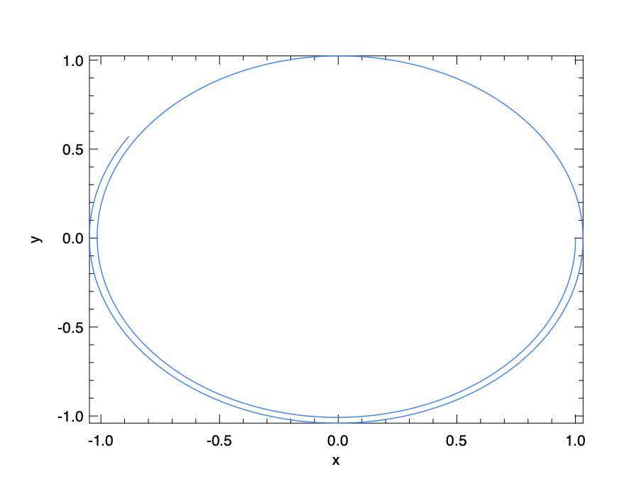
The resulting trajectory by plotting the two components of the ys is show in the figure below. An exact solution would generate a perfect circle, but here we only get a spiral that is similar to a circle. (We have to admit that to better show this effect a large step size is used, but it still exists even using smaller step size.) Aside from improving the solver and precision, is there any other way to solve it better?

Look again at the equation. It shows an interesting pattern: it first uses the value of \(y_1\) to update the \(y_0^{'}\), and then uses \(y_0\) to update the value of \(y_1^{'}\). It belongs to a class of equations that are called the Hamiltonian systems which is often used in the classic mechanics. Such a system is represented by a set of coordinates \((p,q)\). The \(q_i\)’s are called the generalised coordinates, and \(q_i\)’s are corresponding conjugate momenta. The evolution of a Hamiltonian system is defined by the equations below:

\[p' = \frac{\partial{H}}{\partial{q}}, q' = \frac{\partial{H}}{\partial{p}}.\]

Here \(H(p, q)\) is a function of these two components. In the example above, \(p\) and \(q\) are just the two coordinates, and \(H(x,y) = (x^2 + y^2) / 2\). To solve this system, the symplectic solvers are widely used in different fields, since they conserve the value of \(H(p,q)\), to within the order of accuracy of the specific solver used. Most of the usual numerical solvers we have mentioned, such as the Euler and classical RK solvers, are not symplectic solvers.

In Owl_ode we have implemented several symplectic solvers that are based on different integration algorithms: Sym_Euler, Leapfrog, PseudoLeapFrog, Ruth3, and Ruth4. Like the native solvers, they have different orders of error. These algorithms are implemented based on the same basic symplectic integration algorithm, with different parameters. Later we will show an example of using the symplectic solver to solve a damped harmony oscillation problem.

Features and Limits

One feature of owl-ode is the automatic inference of state dimensionality from initial state. For example, the native solvers takes matrix as state. Suppose the initial state of the system is a row vector of dimension \(1\times~N\). After \(T\) time steps, the states are stacked vertically, and thus have dimensions \(T\times~N\). If the initial state is a column vector of shape \(N\times~1\), then the stacked state after \(T\) time steps will be inferred as \(N\times~T\).

The temporal integration of matrices, i.e. cases where the initial state is matrix instead of vector, is also supported. If the initial state is of shape \(N\times~M\), then the accumulated state stacks the flattened state vertically by time steps, which is of shape \(T\times(NM)\). The owl-ode provides a helper function Native.S.to_state_array to unpack the output state into an array of matrices.

Another feature of owl-ode is that the users can easily define new solver module by creating a module of type Solver. For example, to create a custom Cvode solver that has a relative tolerance of 1E-7 as opposed to the default 1E-4, we can define and use the custom_cvode as follows:

let custom_cvode = Owl_ode_sundials.cvode ~stiff:false ~relative_tol:1E-7 ~abs_tol:1E-4
let ts, xs = Owl_ode.Ode.odeint custom_cvode f x0 tspec ()

Here, we use the cvode function to construct a solver module Custom_Owl_Cvode. Similar helper functions like cvode have been also defined for native and symplectic solvers.

We aim to make the owl-ode to run across different backends such as JavaScript. One way to do this is to use tools like js_of_ocaml to convert OCaml bytecode into JavaScript. However, this approach only supports pure OCaml implementation. The sundial and ODEPACK solvers are therefore excluded. Part of the library, the owl-ode-base contains implementations of solvers that are purely written in OCaml. These parts are therefore suitable to be used for in JavaScript and executed on web browsers. Another backend option is the Unikernl virtual machine such as MirageOS. We will talk about these backends in the “Compiler Backends” chapter in the Part II of this book.

One limit of this library is that it is still in a development phase and thus a lot of features is not in place yet. For example, due to the lack of vector-valued root finding functions, we are currently limited to solving initial value problems of explicit ODEs.

Examples of using Owl-ODE

As with many good things in the world, mastering solving ODE requires practice. After getting to know owl-ode, in this section we will demonstrate more examples of using this tool.

Explicit ODE

Now that we have this powerful tool, we can use the solver in owl-ode to solve the motivation problem with simple code.

let f y t = Mat.((2. $* y *$ t) +$ t)

let tspec = Owl_ode.Types.(T1 {t0 = 0.; duration = 1.; dt=1E-3})

let y0 = Mat.zeros 1 1

let solver = Owl_ode.Native.D.rk45 ~tol:1E-9 ~dtmax:10.0

let _, ys = Owl_ode.Ode.odeint solver f y0 tspec ()

The code is mostly similar to previous example, the only difference is that we can now try another solver provided: the rk45 solver, with certain parameters specified. You don’t have to worry about what the tol or dtmax means for now. Note that this solver (and the previous one) requires input to be of type mat in Owl, and the function \(f\) be of type mat -> float -> mat. The result is shown below. You can verify the result by setting the \(x\) to 1 in this equation, and the numerical value of \(y\) will be close to 0.859079.

# Mat.transpose ys
- : Mat.mat =

   C0          C1          C2          C3         C4         C124     C125     C126    C127     C128
R0  0 7.62941E-06 9.91919E-05 0.000251833 0.00046561 ... 0.777984 0.797555 0.817586 0.83809 0.859079

Two Body Problem

In classical mechanics, the two-body problem is to predict the motion of two massive objects. It is assumed that the only force that is considered comes from each other, and both objects are not affected by any other object. This problem can be seen in the astrodynamics where the objects of interests are planets, satellites, etc. under the influence of only gravitation. Another case is the trajectory of electron around Atomic nucleus in a atom.

This classic problem is one of the earliest investigated mechanics problems, and was long solved from the age of Newton. It is also a typical integrable problem in classical mechanics. In this example, let’s consider a simplified version of this problem. We assume that the two objects interact on a 2-dimensional plane, and one of them is so much more massive than the other one that it can be thought of as being static (think about electron and nucleus) and sits at the zero point of a Cartesian coordinate system (0, 0) in the plane. In this system, let’s consider the trajectory of the lighter object. This “one-body” problem is basis of the two body problem. For many forces, including gravitational ones, a two-body problem can be divided into a pair of one-body problems.

Given the previous assumption and newton’s equation, it can be proved that the location of the lighter object [\(y_0\), \(y_1\)] with regard to time \(t\) can be described by:

\[y_0^{''}(t) = -\frac{y_0}{r^3},\] \[y_1^{''}(t) = -\frac{y_1}{r^3},\]

where \(r=\sqrt{y_0^2 + y_1^2}\). This is a second-order ODE system, and to make it solvable using our tool, we need to make it into a first-order explicit ordinary differential equation system:

\[y_0^{'} = y_2,\] \[y_1^{'} = y_3,\] \[y_2^{'} = -\frac{y_0}{r^3},\] \[y_3^{'} = -\frac{y_1}{r^3},\]

Based on the two-system equation, we can build up our code as below:

let f y _t =
  let y = Mat.to_array y in
  let r = Maths.(sqrt ((sqr y.(0)) +. (sqr y.(1)))) in
  let y0' = y.(2) in
  let y1' = y.(3) in
  let y2' = -.y.(0) /. (Maths.pow r 3.) in
  let y3' = -.y.(1) /. (Maths.pow r 3.) in
  [| [|y0'; y1'; y2'; y3'|] |] |> Mat.of_arrays

let y0 = Mat.of_array [|-1.; 0.; 0.5; 0.5|] 1 4
let tspec = Owl_ode.Types.(T1 {t0 = 0.; duration = 20.; dt=1E-2})
let custom_solver = Native.D.rk45 ~tol:1E-9 ~dtmax:10.0

Here the y0 provides initial status of the system: first two numbers denote the initial location of object, and the next two numbers indicate the initial momentum of this object. After building the function, initial status, timespan, and solver, we can then solve the system and visualise it.

let plot () =
  let ts, ys = Ode.odeint custom_solver f y0 tspec () in
  let h = Plot.create "two_body.png" in
  let open Plot in
  plot ~h ~spec:[ RGB (66, 133, 244); LineStyle 1 ] (Mat.col ys 0) (Mat.col ys 1);
  scatter ~h ~spec:[ Marker "#[0x229a]"; MarkerSize 5. ] (Mat.zeros 1 1) (Mat.zeros 1 1);
  text ~h ~spec:[ RGB (51,51,51)] (-.0.3) 0. "Massive Object";
  output h

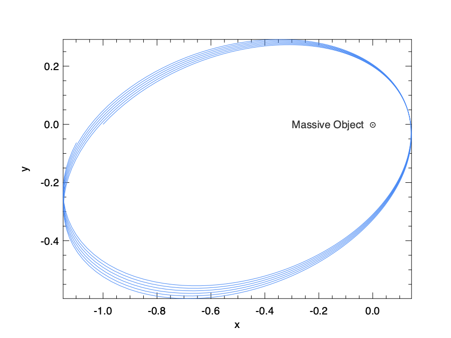
One example of this simplified two-body problem is the “planet-sun” system where a planet orbits the sun. Kepler’s law states that in this system the planet goes around the sun in an ellipse shape, with the sun at a focus of the ellipse. The orbiting trajectory in the result visually follows this theory.

Lorenz Attractor

Lorenz equations are one of the most thoroughly studied ODEs. This system of ODEs is proposed by Edward Lorenz in 1963 to model the flow of fluid (the air in particular) from hot area to cold area. Lorenz simplified the numerous atmosphere factors into the simple equations below.

\[x'(t) = \sigma~(y(t)- x(t))\] \[y'(t) = x(t)(\rho - z(t)) - y(t)\] \[z'(t) = x(t)y(t) - \beta~z(t)\]

Here \(x\) is proportional to the rate of convection in the atmospheric flow; \(y\) and \(z\) are proportional to the horizontal and vertical temperature variation. Parameter \(\sigma\) is the Prandtl number, and \(\rho\) is the normalised Rayleigh number. \(\beta\) is related to the geometry of the domain. The most commonly used parameter values are: \(\sigma = 10, \rho=20\), and \(\beta = \frac{8}{3}\). Based on this information, we can use owl-ode to express the Lorenz equations with code.

let sigma = 10.
let beta = 8. /. 3.
let rho = 28.

let f y _t =
  let y = Mat.to_array y in
  let y0' = sigma *. (y.(1) -. y.(0)) in
  let y1' = y.(0) *. (rho -. y.(2)) -. y.(1) in
  let y2' = y.(0) *. y.(1) -. beta *. y.(2) in
  [| [|y0'; y1'; y2'|] |] |> Mat.of_arrays

We set the initial values of the system to -1, -1, and 1 respectively. The simulation timespan is set to 30 seconds, and the rk45 solver is used.

let y0 = Mat.of_array [|-1.; -1.; 1.|] 1 3
let tspec = Owl_ode.Types.(T1 {t0 = 0.; duration = 30.; dt=1E-2})
let custom_solver = Native.D.rk45 ~tol:1E-9 ~dtmax:10.0

Now, we can solve the ODEs system and visualise the results. In the plots, we first show how the value of \(x\), \(y\) and \(z\) changes with time; next we show the phase plane plots between each two of them.

let _ =
  let ts, ys = Ode.odeint custom_solver f y0 tspec () in
  let h = Plot.create ~m:2 ~n:2 "lorenz_01.png" in
  let open Plot in
  subplot h 0 0;
  set_xlabel h "time";
  set_ylabel h "value on three axes";
  plot ~h ~spec:[ RGB (66, 133, 244); LineStyle 1 ] ts (Mat.col ys 2);
  plot ~h ~spec:[ RGB (219, 68,  55); LineStyle 1 ] ts (Mat.col ys 1);
  plot ~h ~spec:[ RGB (244, 180,  0); LineStyle 1 ] ts (Mat.col ys 0);
  subplot h 0 1;
  set_xlabel h "x-axis";
  set_ylabel h "y-axis";
  plot ~h ~spec:[ RGB (66, 133, 244) ] (Mat.col ys 0) (Mat.col ys 1);
  subplot h 1 0;
  set_xlabel h "y-axis";
  set_ylabel h "z-axis";
  plot ~h ~spec:[ RGB (66, 133, 244) ] (Mat.col ys 1) (Mat.col ys 2);
  subplot h 1 1;
  set_xlabel h "x-axis";
  set_ylabel h "z-axis";
  plot ~h ~spec:[ RGB (66, 133, 244) ] (Mat.col ys 0) (Mat.col ys 2);
  output h

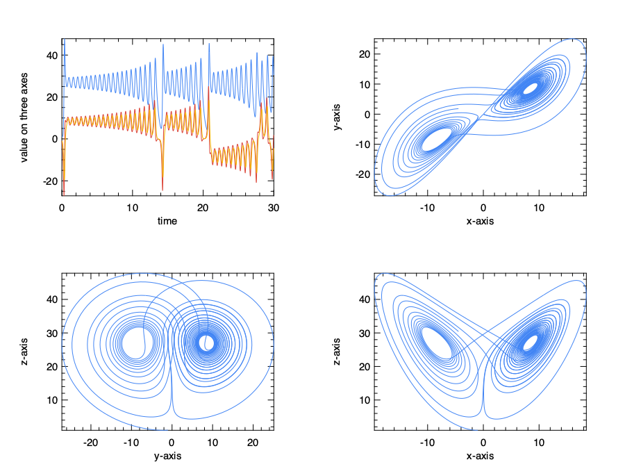
We can imagine that the status of system keep going towards two “voids” in a three dimensional space, jumping from one to the other. These two voids are a certain type of attractors in this dynamic system, where a system tends to evolve towards.

Now, about Lorenz equation, there is an interesting question: “what would happen if I change the initial value slightly?” For some systems, such as a pendulum, that wouldn’t make much a difference, but not here. We can see that clearly with a simple experiment. Keeping function and timespan the same, let’s change only 0.1% of initial value and then solve the system again.

let y00 = Mat.of_array [|-1.; -1.; 1.|] 1 3
let y01 = Mat.of_array [|-1.001; -1.001; 1.001|] 1 3
let ts0, ys0 = Ode.odeint custom_solver f y00 tspec ()
let ts1, ys1 = Ode.odeint custom_solver f y01 tspec ()

To make later calculation easier, we can set the two resulting matrices to be of the same shape using slicing.

let r0, c0 = Mat.shape ys0
let r1, c1 = Mat.shape ys1
let r  = if (r0 < r1) then r0 else r1
let ts = if (r0 < r1) then ts0 else ts1
let ys0 = Mat.get_slice [[0; r-1]; []] ys0
let ys1 = Mat.get_slice [[0; r-1]; []] ys1

Now, we can compare the Euclidean distance between the status of these two systems at certain time. Also, we show the value change of the three components after changing initial values along the time axis.

let _ =
  let h = Plot.create ~m:1 ~n:2 "lorenz_02.png" in
  let open Plot in
  subplot h 0 0;
  set_xlabel h "time";
  set_ylabel h "value on three axes";
  plot ~h ~spec:[ RGB (244, 180,  0); LineStyle 1 ] ts (Mat.col ys1 0);
  plot ~h ~spec:[ RGB (219, 68,  55); LineStyle 1 ] ts (Mat.col ys1 1);
  plot ~h ~spec:[ RGB (66, 133, 244); LineStyle 1 ] ts (Mat.col ys1 2);
  subplot h 0 1;
  let diff = Mat.(
    sqr ((col ys0 0) - (col ys1 0)) +
    sqr ((col ys0 1) - (col ys1 1)) +
    sqr ((col ys0 2) - (col ys1 2))
    |> sqrt
  )
  in
  plot ~h ~spec:[ RGB (66, 133, 244); LineStyle 1 ] ts diff;
  set_xlabel h "time";
  set_ylabel h "distance of two systems";
  output h

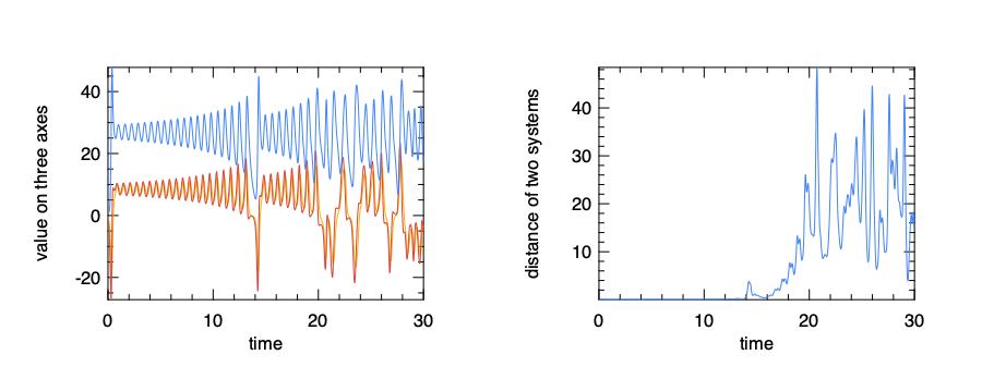
The first figure shows that, initially the systems looks quite like that in the previous figure, but after about 15 seconds, the system state begins to change. This change is then quantified using the Euclidean distance between these two systems. Clearly the difference two system changes sharply after a certain period of time, with no sign of converge. You can try to extend the timespan longer, and the conclusion will still hold.

This result shows that, in the Lorenz system, even a tiny bit of change of the initial state can lead to a large and chaotic change of future state after a while. It partly explains why weather prediction is difficult to do: you can only accurately predict the weather for a certain period of time, any day longer and the weather will be extremely sensitive to a tiny bit of perturbations at the beginning, such as, well, such as the flapping of the wings of a distant butterfly several weeks earlier. You are right, the Lorenz equation is closely related to the idea we now call “butterfly effect” in the pop culture.

Damped Oscillation

This oscillation system appears frequently in Physics and several other fields: charge flow in electric circuit, sound wave, light wave, etc. These phenomena all follow the similar pattern of ODEs. One example is the mass attached on a spring. The system is placed vertically. First the spring stretches to balance the gravity; once the system reaches equilibrium, we can then study the upward displacement of the mass from its original position, denoted with \(x\). One the mass is in motion, at any place \(x\), the pulling force on the mass is proportional to displacement \(x\): \(F=-kx\). Here \(k\) is a positive parameter.

This system is called simple harmonic oscillator, which represents an ideal case where \(F\) is the only force acting on the mass. However, in a real harmonic oscillation system, there is also the frictional force. Such system is called damped oscillation. The frictional force is proportional to the velocity of the mass. Therefore the total force can be expressed as \(F = -kx-cv\). Here \(c\) is the damping coefficient factor. Since both the force and velocity can be expressed as derivatives of \(x\) on time, we have:

\[m\frac{dx}{dt^2} = -kx - c\frac{dx}{dt}\]

Here \(m\) represents the mass of the object. Recall from the previous section that the state of the system in a symplectic solver is a tuple of two matrices, representing the position and momentum coordinates of the system. Therefore, we can express the oscillation equation with a function from this system.

let a = 1.0
let damped_noforcing a (xs, ps) _t : Owl.Mat.mat =
  Owl.Mat.((xs *$ -1.0) + (ps *$ (-1.0 *. a)))

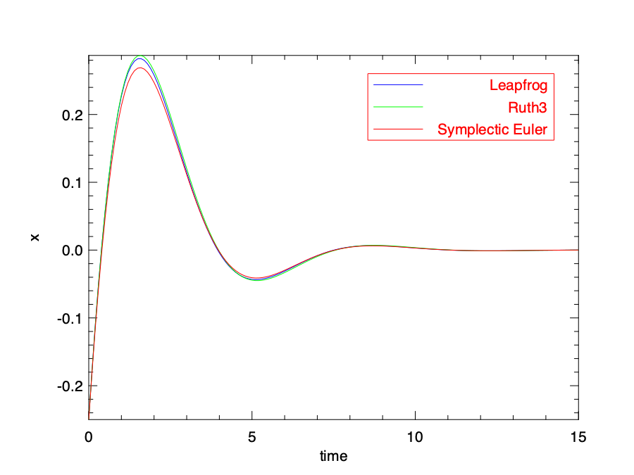
The system evolve function takes the two matrices, position and momentum, and the float number time t as input states. For simplicity, we assume the coefficients are all the same and can be set to one. Let’s then solve with the symplectic solver; we can use the LeapFrog, ruth3, and Symplectic_Euler to compare how their solutions differ.

let main () =
  let x0 = Owl.Mat.of_array [| -0.25 |] 1 1 in
  let p0 = Owl.Mat.of_array [| 0.75 |] 1 1 in
  let t0, duration = 0.0, 15.0 in
  let f = damped_noforcing a in
  let tspec = T1 { t0; duration; dt=0.1 } in
  let t, sol1, _ = Ode.odeint (module Symplectic.D.Leapfrog) f (x0, p0) tspec () in
  let _, sol2, _ = Ode.odeint Symplectic.D.ruth3 f (x0, p0) tspec () in
  let _, sol3, _ =
    Ode.odeint (module Symplectic.D.Symplectic_Euler) f (x0, p0) tspec ()
  in
  t, sol1, sol2, sol3

You should be familiar with this code by now. It defines the initial values, the time duration, time step, and then provides this information to the solvers. Unlike native solvers, these symplectic solvers return three values instead of two: the first is the time sequence, and the next two sequences indicate how the \(x\) and \(p\) values evolve at each time point.

let plot_sol fname t sol1 sol2 sol3 =
  let h = Plot.create fname in
  let open Plot in
  plot ~h ~spec:[ RGB (0, 0, 255); LineStyle 1 ] t (Mat.col sol1 0);
  plot ~h ~spec:[ RGB (0, 255, 0); LineStyle 1 ] t (Mat.col sol2 0);
  plot ~h ~spec:[ RGB (255, 0, 0); LineStyle 1 ] t (Mat.col sol3 0);
  set_xlabel h "time";
  set_ylabel h "x";
  legend_on h ~position:NorthEast [| "Leapfrog"; "Ruth3"; "Symplectic Euler" |];
  output h

Here we only plot the change of position \(x\) over time in the oscillation, and plot the solution provided by the three different solvers, as shown in the plotting code above. You can also try to visualise the change to the momentum \(p\) in a similar way. The result is shown in the figure below. You can clearly see that the displacement decreases towards equilibrium position in this damped oscillation as the energy dissipating. The curves provided by three solvers are a bit different, especially at the peak of the curve, but keep close enough for most of the time.

Stiffness

Stiffness is an important concept in the numerical solution of ODE. Think about a function that has a “cliff” where at a point its nearby value changes rapidly. To find the solution with normal method as we have used, it may requires such an extremely small stepping size that traversing the whole timespan may takes a very long time and lot of computation. Therefore, the solver of stiff equations needs to use different methods such as implicit differencing or automatic step size adjustment etc. to keep it accurate and robust.

The Van der Pol equation is a good example to show both non-stiff and stiff cases. In dynamics, the Van der Pol oscillator is a non-conservative oscillator with non-linear damping. Its behaviour with time can be described with a high order ODE:

\[y^{''} - \mu~(1-y^2)y' + y = 0,\]

where \(\mu\) is a scalar parameter indicating the non-linearity and the strength of the damping. To make it solvable using our tool, we can change it into a pair of explicit one-order ODEs in a linear system:

\[y_0^{'} = y_1,\] \[y_1^{'} = \mu~(1-y_0^2)y_1 - y_0.\]

As we will show shortly, by varying the damping parameter, this group of equations can be either non-still or stiff.

We provide both stiff (Owl_Cvode_Stiff) and non-still (Owl_Cvode) solvers by interfacing to Sundials, and the LSODA solver of ODEPACK can automatically switch between stiff and non-stiff algorithms. We will try both in the example. We start with the basic function definition code that are shared by both cases:

open Owl_ode
open Owl_ode.Types
open Owl_plplot

let van_der_pol mu =
  fun y _t ->
    let y = Mat.to_array y in
    [| [| y.(1); mu *. (1. -. Maths.sqr y.(0)) *. y.(1) -.y.(0) |] |]
    |> Mat.of_arrays

Solve Non-Stiff ODEs

When set the parameter to 1, the equation is a normal non-stiff one, and let’s try to use the Cvode solver from sundials to do this job.

let f_non_stiff = van_der_pol 1.

let y0 = Mat.of_array [| 0.02; 0.03 |] 1 2

let tspec = T1 { t0 = 0.0; dt = 0.01; duration = 30.0 }

let ts, ys = Ode.odeint (module Owl_ode_sundials.Owl_Cvode) f_stiff y0 tspec ()

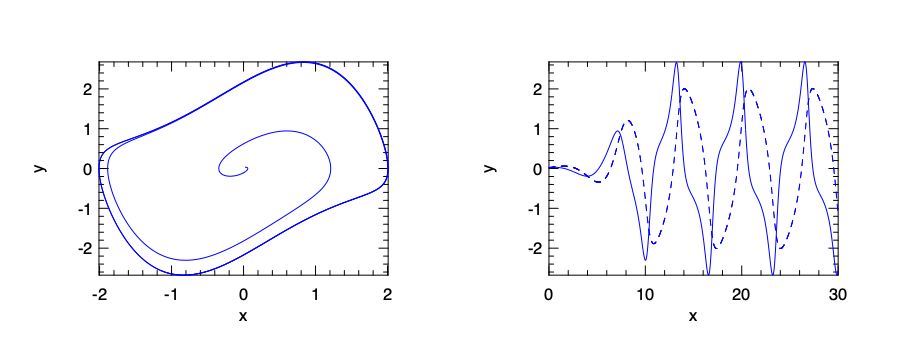
Everything seems normal. To see the “non-stiffness” clearly, we can plot how the two system states change over time, and a phase plane plot of their trajectory on the plane, using the two states as x- and y-axis values. The result is shown below.

let () =
  let fname = "vdp_sundials_nonstiff.png" in
  let h = Plot.create ~n:2 ~m:1 fname in
  let open Plot in
  set_foreground_color h 0 0 0;
  set_background_color h 255 255 255;
  subplot h 0 0;
  plot ~h ~spec:[ RGB (0, 0, 255); LineStyle 1 ] (Mat.col ys 0) (Mat.col ys 1);
  subplot h 0 1;
  plot ~h ~spec:[ RGB (0, 0, 255); LineStyle 1 ] ts Mat.(col ys 1);
  plot ~h ~spec:[ RGB (0, 0, 255); LineStyle 3 ] ts Mat.(col ys 0);
  output h

Solve Stiff ODEs

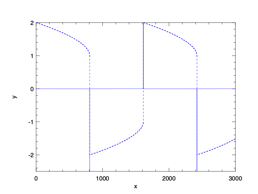
Change the parameters to 1000, and now this function becomes stiff. We follow the same procedure as before, but now we use the Lsoda solver from odepack, and the timespan is extended to 3000. We can see clearly what “stiff” means. Both lines in this figure contain very sharp “cliffs”.

let f_stiff = van_der_pol 1000.
let y0 = Mat.of_array [| 2.; 0. |] 1 2
let tspec = T1 { t0 = 0.0; dt = 0.01; duration = 3000.0 }

let () =
  let ts, ys = Ode.odeint (module Owl_ode_odepack.Lsoda) f_stiff y0 tspec () in
  let fname = "vdp_odepack_stiff.png" in
  let h = Plot.create fname in
  let open Plot in
  set_foreground_color h 0 0 0;
  set_background_color h 255 255 255;
  set_yrange h (-2.) 2.;
  plot ~h ~spec:[ RGB (0, 0, 255); LineStyle 1 ] ts Mat.(col ys 1);
  plot ~h ~spec:[ RGB (0, 0, 255); LineStyle 3 ] ts Mat.(col ys 0);
  output h

Summary

This chapter discusses solving the initial value problem of ordinary differential equations (ODEs) numerically. We first present the general definition of the ODE and the initial value problem. There are already many existing mathematical solution to ODEs of certain format, but that is not the focus of this chapter. This chapter is centred on the owl-ode library. It implements several native and symplectic solvers. We have briefly explained the basic idea of these methods. Also, this library interfaces to existing off-the-shelf open source ODE solvers from the Sundials and ODEPACK library. Next, we demonstrate how these solvers are used to solve ODE from several real examples, including the Two-body problem, the Lorentz Attractor, and Damped Oscillation, etc. Finally, we introduce one important idea in the solving ODE numerically: stiffness, and then shows how we can solve stiff and non-stiff ODEs with the example of the van der pol equation. Hopefully, after studying this chapter, the readers can have a basic idea of how numerical ODE solver works and how to apply them into solving real-world problems.