CHAPTER 08
Algorithmic Differentiation
Differentiation is core to many scientific applications including maximising or minimising functions, solving systems of ODEs, and non-linear optimisation, including the evaluation of derivatives in KKT optimality conditions. Algorithmic differentiation (AD) is a computer-friendly technique for performing differentiation that is both efficient and accurate. An important application of algorithmic differentiation is in machine learning and artificial intelligence. [1] Gradient-based neural network training evaluates a loss in a forward pass, computes its derivatives with respect to the parameters by backpropagation, and then updates the parameters. [2] In this chapter, we will introduce this topic using a hands-on approach. Starting from the basic definition, we build up a simplified AD engine step by step. We then move to the AD engine in Owl to present its usage and more implementation details.
8.1 Chain Rule
We often need to study the functional relationship between variables: how much one variable changes when the value of another variable changes. For example, assume an object moving along a line has a displacement of in a time . We can define the velocity describing the motion of the object as the ratio of displacement in a given time as the time considered gets smaller and smaller, eventually approaching zero:
| (8.1) |
The term is referred to as “the derivative of with respect to ”.
We can extend this to higher dimensional spaces. For example, we might try to describe the temperature distribution in a solid material that has not been heated evenly. The temperature of a point in the material can be modelled as a function of that point’s Cartesian coordinates , and we can consider how the temperature changes with position within the material as shown in Eq. 8.2 [3].
| (8.2) |
The vector is referred to as “the gradient of ”. Because might vary differently with respect to the different quantities , , , we refer to as “the partial derivative with respect to ”.
In general, the process of calculating derivatives and gradients is referred to as differentiation. [4] Although some differentiation involves complex manipulations and may seem daunting, the underlying procedures are often quite mechanical. One particularly important such procedure is called the chain rule, used to calculate the derivative of a composite function. [4]
Suppose we have two functions and that can be composed to create a function . The chain rule states that the derivative of can be calculated as:
| (8.3) |
This seemingly simple rule is one of the most fundamental rules in calculating derivatives. For example, let , where is a real number and , and we can obtain using the chain rule by rewriting and setting so that we have . Applying the chain rule gives
Tbl. 8.1 summarises how to apply the chain rule when composing functions using basic operations such as addition and multiplication, where is a variable, and are functions of , and is a constant. These equations are like the building blocks used to differentiate more complex functions. For the logarithms, and the base satisfies , ; the quotient rule requires . Armed with the chain rule and these basic equations, we can solve a wide range of problems.
8.2 Differentiation Methods
As functions become more complicated, manual differentiation becomes both tedious and error-prone. Fortunately, we can use computers to automate the process and there are three different ways that are widely used to do so: numerical differentiation, symbolic differentiation, and algorithmic differentiation.
8.2.1 Numerical Differentiation
Arising directly from the definition of derivative in Eq. 8.1, numerical differentiation uses a small step to compute an approximate value for the limit in the definition
| (8.4) |
The resulting approximation uses four steps: (i) evaluate the given at point ; (ii) choose a suitable small and add it to the original ; (iii) re-evaluate the function at ; and (iv) evaluate the finite quotient, without taking the limit in Eq. 8.4. By treating the function as a black box, then this method is straightforward to implement as long as can be evaluated, but is unfortunately subject to errors including truncation and round-off error. [5]
Truncation error is the error caused by approximating a mathematical process. The limit in Eq. 8.4 defines the exact derivative, but a nonzero step gives an approximation. For a twice continuously differentiable function and , the Taylor expansion with remainder gives:
Here is the step size and is in the range of . This equation can be manipulated into
The term is the exact derivative minus its forward-difference approximation, an error of order . For example, if then and if we calculate the derivative at numerically using a step size of , then the truncation error will be in the range .
Step size directly affects the truncation error, as can be seen by considering the effect of using a very large step size. For example, we wish to find the derivative of at point . The analytical solution gives the value but the numerical result deviates substantially from that actual value, as shown by the code below.
# let d =
      let _eps = 0.1 in
      let diff f x = (f (x +. _eps) -. f x) /. _eps in
      diff Owl_maths.cos 1.;;
val d : float = -0.867061844425624506
Round-off error is caused by representing numbers with only finite precision during the numerical computation. Looking back at Eq. 8.4 we need to calculate , i.e. to subtract two numbers that are almost equal which can lead to large round-off errors. For example, consider using a very small step size to avoid truncation error
# let d =
      let _eps = 5E-16 in
      let diff f x = (f (x +. _eps) -. f x) /. _eps in
      diff Owl_maths.cos 1.;;
val d : float = -0.888178419700125121
Again, this result deviates substantially from the actual value. Indeed, if we were to use an even smaller step size, , the result actually becomes : in this calculation, rounds to , so the subtraction returns zero.
Finally, computing a full gradient by coordinate-wise finite differences requires repeated evaluations of , which can be expensive in many dimensions. Numerical differentiation is straightforward to implement, but choosing the step size involves a trade-off between truncation and round-off error, and the cost depends on the function and the number of derivatives required.
8.2.2 Symbolic Differentiation
By manipulating the underlying mathematical expressions, symbolic differentiation obtains analytical results without numerical approximation, using rules such as those introduced in Tbl. 8.1. For example, consider the function . Computing symbolically, we end up with:
This gives an exact derivative expression, although evaluating it numerically still incurs round-off. The complexity of symbolic manipulation can grow as expressions become more complex: try using symbolic differentiation to compute the derivative of to test if that is true! You will quickly realise that symbolic computations may generate many very complex intermediate results, even for quite simple functions. As a result, symbolic differentiation can easily consume a huge amount of memory and CPU cycles.
In addition, in contrast to numerical differentiation, we must treat the function we are differentiating as a white box, and know exactly what is inside of it. This further increases the difficulty of using symbolic differentiation to derive arbitrary functions, although it can generate exact derivative expressions. [6]
8.2.3 Algorithmic Differentiation
A chain-rule based technique for calculating derivatives with respect to input variables of functions defined in a computer programme, algorithmic differentiation (AD) is also known as automatic differentiation, though strictly speaking it does not fully automate differentiation and can sometimes lead to inefficient code. [7] [8]
In general though, AD efficiently evaluates derivatives by applying exact differentiation rules to the operations executed by a program. It avoids finite-difference truncation error, but remains subject to floating-point round-off and the availability of valid derivative rules. It differs from finite differences and from constructing a symbolic derivative expression, and scales well to many real world applications. [9] Griewank [10] gives a bound of five times the arithmetic cost of evaluating a scalar function for computing its gradient by reverse mode, under the operation-counting model used in that analysis. This is not a universal wall-clock bound for every implementation. Implementations of AD have appeared in many languages, including Python [11], Julia [12], and MATLAB [13]. The rest of this chapter introduces AD. [14] [15]
8.3 How Algorithmic Differentiation Works
We start by showing how AD works using an example. We have seen how the chain rule can be applied to simple functions such as , so now let us consider a more complicated function based on a sigmoid function
| (8.5) |
We wish to compute . To illustrate this process we represent Eq. 8.5 as the computation graph shown in Fig. 8.1. At the right side of the figure is the final output , and the roots of this graph are the input variables on the left side of the figure. The nodes between them are either constants or intermediate variables produced by the mathematical functions such as sine. All nodes are labelled , and an edge between two nodes indicates a dependency in the computation.
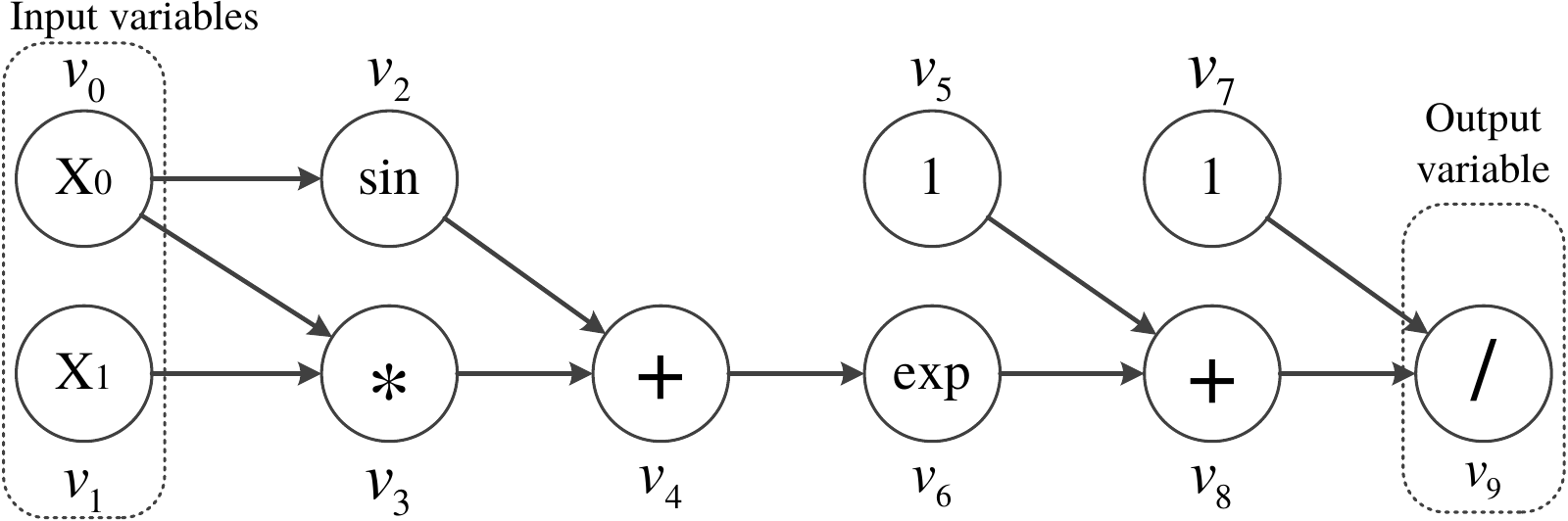
Considering this graphical representation, there are two ways to apply the chain rule: forward mode and reverse mode.
1 We next consider each in turn.
8.3.1 Forward Mode
We ultimately wish to calculate (and , which follows similarly) but we will begin by calculating some intermediate results that will prove to be useful. Using the labels to refer to the intermediate computations, we have and immediately. Next, consider , which is a bit trickier and requires use of the chain rule
After calculating , we proceed to compute partial derivatives of , , and so on to which will give us the final result we are looking for. This process starts with the input variables and ends with the output variables and so is called forward differentiation.2
We can simplify the notation by letting . The is called the tangent of the function with respect to the input variable , and the results of evaluating the function at each intermediate point are called primal value.
Let’s calculate when setting , and . The full forward differentiation calculation process is shown in Tbl. 8.2 where two simultaneous computation processes take place in the two computation columns: (i) the primal computation is the procedure defined by Eq. 8.5; and (ii) the tangent computation gives the derivative for each intermediate variable with regard to .
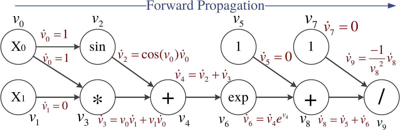
The procedure in Tbl. 8.2 is illustrated in Fig. 8.2. We can validate this result
with the algorithmic differentiation module Algodiff in Owl. Don’t worry if you
don’t understand the code at the moment! We will cover the details later in this
chapter.
# open Algodiff.D;;

# let f x =
      let x1 = Mat.get x 0 0 in
      let x2 = Mat.get x 0 1 in
      Maths.(div (F 1.) (F 1. + exp (x1 * x2 + (sin x1))));;
val f : Owl_algodiff.D.t -> Owl_algodiff.D.t = <fun>
# let x = Mat.ones 1 2;;
val x : Owl_algodiff.D.t = Owl_algodiff.D.Arr
   C0 C1
R0  1  1
# let _ = grad f x |> unpack_arr;;
- : Owl.Algodiff.D.A.arr =
          C0        C1
R0 -0.181974 -0.118142
The first value in the output ndarray -0.181974 verifies our manual calculation
in the table.
8.3.2 Reverse Mode
Let us now think about this problem in the other direction, from outputs to inputs. The problem remains the same, i.e. to calculate , and we will still follow the same “step by step” idea from forward mode – only that we will just calculate it backwards. For example, the graph shows that so if we only knew and , we would have taken a step towards our target solution.
We first observe that , as and are identical. We then compute by applying the chain rule
| (8.6) |
This looks complex but we can simplify by applying a substitution
for the derivative of output variable with regard to intermediate node . is called “the adjoint of variable with respect to the output variable ”. Using this notation, Eq. 8.6 can be rewritten
Note the difference between tangent and adjoint. In forward mode, we know and and then calculate , , …until we get the target . In reverse mode, we start with and calculate , , …until we have , our target. Again, in this example, given that we are talking about derivative with respect to when we use . As a result, reverse mode is also called adjoint mode.
With that in mind, we can now follow the complete reverse differentiation procedure. We first perform a forward pass, shown in Tbl. 8.3, to compute the required intermediate values identical to those in the Primal Computation column of Tbl. 8.2.
Note that is used in both intermediate variables and so we compute the contributions to the adjoint of through (step 19) and (step 20), before adding them together (step 21).
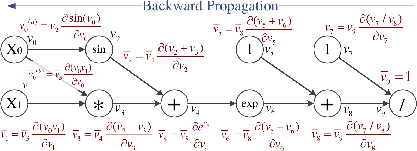
As with forward mode, Fig. 8.3 depicts the reverse differentiation process in Tbl. 8.4. This result agrees with the result when using forward mode. We can also use Owl to perform a numerical differentiation to further validate, and the code is similar to that of using algorithmic differentiation as shown above.
open Owl;;
module D = Owl_numdiff_generic.Make (Dense.Ndarray.D);;
let x = Arr.ones [|2|];;
let f x =
  let x1 = Arr.get x [|0|] in
  let x2 = Arr.get x [|1|] in
  Maths.(div 1. (1. +. exp (x1 *. x2 +. (sin x1))));;
Then we can get the result of the differentiation at the point , which again agrees with both the previous results using the AD module and our table-based calculation.
# D.grad f x;;
- : Owl.Dense.Ndarray.D.arr =
         C0        C1
R -0.181973 -0.118142
Before we continue it is worth noting that we obtained “for free” while calculating in reverse mode. This observation will be used in the next section where we discuss how to decide whether to use forward or reverse mode in practice.
8.3.3 Forward Mode or Reverse Mode?
As both can be used to differentiate functions there is a natural question over which should be used in practice. Inevitably, the short answer is: it depends. However, a useful rule of thumb is
- if the number of input variables is far greater than that of the output variables, then use reverse mode; whereas
- if the number of output variables is far greater than that of the input variables, then use forward mode.
For a full Jacobian, basic forward mode uses one coordinate seed per input, while reverse mode uses one output seed per output component. Each reverse pass gives derivatives of that selected output with respect to all inputs; for a scalar output, one reverse pass gives the full gradient. This is particularly relevant when training deep neural networks: the differentiated inputs are the many model parameters, and the output is a scalar loss. If only a directional derivative or a Jacobian-vector product is needed, the number of required seeds changes.
The trade-off is that reverse mode needs access to intermediate values for its backward pass, usually by recording a graph or tape, or by recomputing values. Forward mode propagates tangents alongside primal values and does not require a reverse tape. We will show another example of choosing between these two methods later in this chapter.
8.4 A Strawman AD Engine
Clearly you would not want to produce these tables every time you had a new function to differentiate! Far better to let the computer do it – and the “how” is the topic of this section. We will discuss how to implement both differentiation modes in OCaml, albeit using considerably simplified implementations compared to the AD module in Owl.
We will once more use the function in Eq.8.5 as an example, and limit the
computations supported by our small AD engine to just sine (sin), exponential
(exp), addition (add), division (div), and multiplication (mul).
8.4.1 Implementation of Forward Mode
Tbl. 8.2 shows that an intermediate node actually needs to know only the primal and tangent values of its parents’ nodes to compute its own results. Using this observation we define a data type to track these two values:
type df = {
  mutable p: float;
  mutable t: float;
};;

let primal df = df.p;;
let tangent df = df.t;;
We next define operators that take values of type df as input, and produce values
of type df as output. In each case, we must define how to compute the function value
p’ and derivative value t’ given the input data df. Calculation of derivatives is
based on rules such as those listed in Tbl. 8.1. For example, for sin and
exp:
let sin_ad x =
  let p = primal x in
  let t = tangent x in
  let p' = Owl_maths.sin p in
  let t' = (Owl_maths.cos p) *. t in
  {p = p'; t = t'};;
let exp_ad x =
  let p = primal x in
  let t = tangent x in
  let p' = Owl_maths.exp p in
  let t' = p' *. t in
  {p = p'; t = t'};;
Operators that accept multiple inputs require a little more thought but essentially the same procedure. First, addition:
let add_ad a b =
  let pa = primal a in
  let ta = tangent a in
  let pb = primal b in
  let tb = tangent b in
  let p' = pa +. pb in
  let t' = ta +. tb in
  {p=p'; t=t'};;
Then multiplication and division:
let mul_ad a b =
  let pa = primal a in
  let ta = tangent a in
  let pb = primal b in
  let tb = tangent b in
  let p' = pa *. pb in
  let t' = pa *. tb +. ta *. pb in
  {p = p'; t = t'};;
let div_ad a b =
  let pa = primal a in
  let ta = tangent a in
  let pb = primal b in
  let tb = tangent b in
  let p' = pa /. pb in
  let t' = (ta *. pb -. tb *. pa) /. (pb *. pb) in
  {p=p'; t=t'};;
Having defined these functions, we next create a tiny wrapper named
diff
let diff f =
  let f' x y =
    let r = f x y in
    primal r, tangent r
  in
  f';;
...and that’s all! We can now differentiate our previous example, starting with the
inputs for which we know the tangent of x1 with regard to x0 is zero, as are the other
constants used in the computation, while the tangent of x0 with regard to itself is, of
course, one.
let x0 = {p=1.; t=1.};;
let x1 = {p=1.; t=0.};;
We then simply define our function f in terms of the operations given above, and
apply our diff function
# let f x0 x1 =
    let v2 = sin_ad x0 in
    let v3 = mul_ad x0 x1 in
    let v4 = add_ad v2 v3 in
    let v5 = {p=1.; t=0.} in
    let v6 = exp_ad v4 in
    let v7 = {p=1.; t=0.} in
    let v8 = add_ad v5 v6 in
    let v9 = div_ad v7 v8 in
    v9;;
val f : df -> df -> df = <fun>
# let p, t = diff f x0 x1;;
val p : float = 0.13687741466075895
val t : float = -0.181974376561731321
The resulting t, ,
is equal to that calculated earlier.
8.4.2 Implementation of Reverse Mode
Reverse mode is slightly more complex. As the previous section illustrated, forward mode needs only one pass while reverse mode requires two – a forward pass followed by a backward pass. Thus, as well as computing the primal values in the forward pass, we must also record the operations applied so we can use them in the backward pass. There are many ways this could be done, e.g., using a stack or a graph, but here we use a different approach. As ever, we begin with our data types.
type dr = {
  mutable p: float;
  mutable a: float ref;
  mutable adj_fun : float ref ->
    (float * dr) list -> (float * dr) list
};;

let primal dr = dr.p;;
let adjoint dr = dr.a;;
let adj_fun dr = dr.adj_fun;;
It is hopefully easy enough to understand p as the primal and a as the adjoint,
but the adj_fun is a little more complex so we will illustrate it with an example
implementing the sin operation
let sin_ad dr =
  let p = primal dr in
  let p' = Owl_maths.sin p in
  let adjfun' ca t =
      let r = !ca *. (Owl_maths.cos p) in
      (r, dr) :: t
  in
  {p=p'; a=ref 0.; adj_fun=adjfun'};;
The adj_fun is a callback that will propagate an adjoint contribution once it is
available, while t is a stack of intermediate nodes yet to be processed in the
backward pass. One way to read this definition is as saying that once we have the
adjoint value ca, we can compute an adjoint contribution for the parent r by
following the derivative calculation rules and the chain rule. This result, together
with the original data dr, is pushed onto the stack t (naively implemented as an
OCaml list).
Next, we consider mul, an operation with two variables
let mul_ad dr1 dr2 =
  let p1 = primal dr1 in
  let p2 = primal dr2 in
  let p' = Owl_maths.mul p1 p2 in
  let adjfun' ca t =
      let r1 = !ca *. p2 in
      let r2 = !ca *. p1 in
      (r1, dr1) :: (r2, dr2) :: t
  in
  {p = p'; a = ref 0.; adj_fun = adjfun'};;
For this operation, both parents must be added to the task stack t as
multiplication has two inputs. We also need a helper function to encapsulate input
data
let make_reverse v =
  let a = ref 0. in
  let adj_fun _a t = t in
  {p=v; a; adj_fun};;
With this we can now perform a forward pass on a simple example , evaluated at .
# let x = make_reverse 1.;;
val x : dr = {p = 1.; a = {contents = 0.}; adj_fun = <fun>}
# let y = make_reverse 2.;;
val y : dr = {p = 2.; a = {contents = 0.}; adj_fun = <fun>}
# let v = mul_ad (sin_ad x) y;;
val v : dr = {p = 1.68294196961579301; a = {contents = 0.}; adj_fun = <fun>}
At this point, after the forward pass for this smaller example, we have
the primal values at each intermediate node but all their adjoint values are
zero as they have not yet been calculated. To perform the analogous reverse
pass, we need two sets of information: the forward calculation values, and
how to calculate the derivatives. The first is stored in the dr.p field, and
the second is stored in the adj_fun. We thus need a recursive function,
reverse_push, that can use these sets of information to complete the reverse pass
calculations.
let rec reverse_push = function
  | [] -> ()
  | (v, dr) :: t ->
      let aa = adjoint dr in
      let adjfun = adj_fun dr in
      aa := !aa +. v;
      let stack = adjfun (ref v) t in
      reverse_push stack;;

let reverse_reset roots =
  let seen = ref [] in
  let rec visit dr =
    let a = adjoint dr in
    if not (List.exists (fun b -> a == b) !seen) then (
      seen := a :: !seen;
      a := 0.;
      List.iter (fun (_, parent) -> visit parent) (adj_fun dr (ref 0.) []))
  in List.iter visit roots;;
Each pending edge carries an adjoint increment. We accumulate it at the node, but propagate only that increment; propagating the accumulated value again would double-count shared intermediate nodes. Before each differentiation, we reset the adjoints of the reachable graph.
Given the calculations recorded in the forward pass, reverse_push works
backwards through the pending contributions. It removes a pair (v, dr) from the
list and adds v to the node’s adjoint accumulator aa. It then passes ref v, not
the accumulated aa, to adj_fun, which pushes the resulting contributions
and parent nodes onto the stack. This step is repeated until the stack is
empty.
The other operations required by Eq. 8.5 follow similarly
let exp_ad dr =
  let p = primal dr in
  let p' = Owl_maths.exp p in
  let adjfun' ca t =
      let r = !ca *. (Owl_maths.exp p) in
      (r, dr) :: t
  in
  {p=p'; a=ref 0.; adj_fun=adjfun'};;

let add_ad dr1 dr2 =
  let p1 = primal dr1 in
  let p2 = primal dr2 in
  let p' = Owl_maths.add p1 p2 in
  let adjfun' ca t =
    let r1 = !ca in
    let r2 = !ca in
    (r1, dr1) :: (r2, dr2) :: t
  in
  {p = p'; a = ref 0.; adj_fun = adjfun'};;

let div_ad dr1 dr2 =
  let p1 = primal dr1 in
  let p2 = primal dr2 in
  let p' = Owl_maths.div p1 p2 in
  let adjfun' ca t =
      let r1 = !ca /. p2 in
      let r2 = !ca *. (-.p1) /. (p2 *. p2) in
      (r1, dr1) :: (r2, dr2) :: t in
  {p = p'; a = ref 0.; adj_fun = adjfun'};;
We can then write the reverse mode differentiation function diff that runs a
forward pass followed by a backward pass
let diff f =
  let f' x =
    let r = f x in (* the forward pass *)
    reverse_reset [r];
    reverse_push [(1., r)]; (* the backward pass *)
    let x0, x1 = x in
    primal x0, !(adjoint x0), primal x1, !(adjoint x1)
  in f';;
We can then derive the function for reverse mode differentiation
let f (x0, x1) =
  let v2 = sin_ad x0 in
  let v3 = mul_ad x0 x1 in
  let v4 = add_ad v2 v3 in
  let v5 = make_reverse 1. in
  let v6 = exp_ad v4 in
  let v7 = make_reverse 1. in
  let v8 = add_ad v5 v6 in
  let v9 = div_ad v7 v8 in
  v9;;
Finally, with all these parts to hand, we can perform the differentiation having encapsulated the input variables, in just three lines of code. Again, the resulting adjoint values are just as expected.
# let x1 = make_reverse 1.;;
val x1 : dr = {p = 1.; a = {contents = 0.}; adj_fun = <fun>}
# let x0 = make_reverse 1.;;
val x0 : dr = {p = 1.; a = {contents = 0.}; adj_fun = <fun>}
# let pri_x0, adj_x0, pri_x1, adj_x1 = diff f (x0, x1);;
val pri_x0 : float = 1.
val adj_x0 : float = -0.181974376561731321
val pri_x1 : float = 1.
val adj_x1 : float = -0.118141988016545588
8.4.3 A Unified Implementation
We have shown how to implement forward and reverse AD separately, from
scratch, but we often need a system that supports both modes. We start by
combining the record type df and variant type dr into a new data type t with the
accompanying operations:
type t =
  | DF of float * float
  | DR of float * float ref * adjoint
and adjoint = float ref -> (float * t) list -> (float * t) list

let primal = function
  | DF (p, _) -> p
  | DR (p, _, _) -> p

let tangent = function
  | DF (_, t) -> t
  | DR (_, _, _) -> failwith "error: no tangent for DR"

let adjoint = function
  | DF (_, _) ->  failwith "error: no adjoint for DF"
  | DR (_, a, _) -> a;;
We then give functions to pack the variables of both modes into the same type t
so that we can write a unified differentiation function.
let make_forward p a = DF (p, a)

let make_reverse p =
    let a = ref 0. in
    let adj_fun _a t = t in
    DR (p, a, adj_fun)

let rec reverse_push = function
  | [] -> ()
  | (v, x) :: t ->
    (match x with
     | DR (_, a, adjfun) ->
       a := !a +. v;
       let stack = adjfun (ref v) t in
       reverse_push stack
     | _ -> failwith "error: unsupported type");;

let reverse_reset roots =
  let seen = ref [] in
  let rec visit = function
    | DF _ -> ()
    | DR (_, a, adjfun) ->
      if not (List.exists (fun b -> a == b) !seen) then (
        seen := a :: !seen;
        a := 0.;
        List.iter (fun (_, parent) -> visit parent) (adjfun (ref 0.) []))
  in List.iter visit roots;;
Using this new data type, we can then simply combine the previous forward and reverse mode implementations into a single function using pattern matching. For example, the sin function becomes
let sin_ad x =
  let ff = Owl_maths.sin in
  let df p t = (Owl_maths.cos p) *. t in
  let dr p a = !a *. (Owl_maths.cos p) in
  match x with
  | DF (p, t) ->
    let p' = ff p in
    let t' = df p t in
    DF (p', t')
  | DR (p, _, _) ->
    let p' = ff p in
    let adjfun' a t =
      let r = dr p a in
      (r, x) :: t
    in
    DR (p', ref 0., adjfun');;
Similarly, for the multiplication operator
let mul_ad xa xb =
  let ff = Owl_maths.mul in
  let df pa pb ta tb = pa *. tb +. ta *. pb in
  let dr pa pb a = !a *. pb, !a *. pa in
  match xa, xb with
  | DF (pa, ta), DF (pb, tb) ->
    let p' = ff pa pb in
    let t' = df pa pb ta tb in
    DF (p', t')
  | DR (pa, _, _), DR (pb, _, _) ->
    let p' = ff pa pb in
    let adjfun' a t =
      let ra, rb = dr pa pb a in
      (ra, xa) :: (rb, xb) :: t
    in
    DR (p', ref 0., adjfun')
  | _, _ -> failwith "unsupported op";;
While this approach certainly works, it rapidly becomes clear that we are writing a considerable amount of boilerplate code. This is generally worth avoiding, something that OCaml’s powerful mechanisms for abstraction can often help to achieve. So, before moving on, let us take a moment to think about how to categorise different math functions to see if we can find some structure to exploit to allow us to stop writing so much boilerplate code.
One way to categorise maths functions is by their arity, namely the number of input variables. Some are unary (one input, e.g., sin x), some are binary functions (two inputs, e.g., mul x y), and so on. Each shares an identical code structure and we can use OCaml’s powerful module system to abstract over all operations of a given arity to avoid writing too much boilerplate code.
We will express each operation as an OCaml module, containing three core
operations: (i) ff, to calculate the primal value of the function; (ii) df, to calculate
the tangent value in the forward mode; and (iii) dr, to calculate the adjoint value in
the reverse mode. The following code uses sin and mul as examples of unary and
binary operations
module type Unary = sig
  val ff : float -> float
  val df : float -> float -> float
  val dr : float -> float ref -> float
end
module type Binary = sig
  val ff : float -> float -> float
  val df : float -> float -> float -> float -> float
  val dr : float -> float -> float ref -> float * float
end

module Sin = struct
  let ff = Owl_maths.sin
  let df p t = (Owl_maths.cos p) *. t
  let dr p a = !a *. (Owl_maths.cos p)
end

module Mul = struct
  let ff = Owl_maths.mul
  let df pa pb ta tb = pa *. tb +. ta *. pb
  let dr pa pb a = !a *. pb, !a *. pa
end;;
Modules of different arity need their own functions to calculate primal, tangent, and adjoint values, which we can provide using modules as parameters
let unary_op (module U: Unary) = fun x ->
  match x with
  | DF (p, t) ->
    let p' = U.ff p in
    let t' = U.df p t in
    DF (p', t')
  | DR (p, _, _) ->
    let p' = U.ff p in
    let adjfun' a t =
      let r = U.dr p a in
      (r, x) :: t
    in
    DR (p', ref 0., adjfun')


let binary_op (module B: Binary) = fun xa xb ->
  match xa, xb with
  | DF (pa, ta), DF (pb, tb) ->
    let p' = B.ff pa pb in
    let t' = B.df pa pb ta tb in
    DF (p', t')
  | DR (pa, _, _), DR (pb, _, _) ->
    let p' = B.ff pa pb in
    let adjfun' a t =
      let ra, rb = B.dr pa pb a in
      (ra, xa) :: (rb, xb) :: t
    in
    DR (p', ref 0., adjfun')
  | _, _ -> failwith "unsupported op";;
Each such function takes a module as input and returns a function that can be used in either forward or backward mode. This procedure is performed with a concise line of code for each operation. Using our sin and mul examples from before
let sin_ad = unary_op (module Sin : Unary)
let mul_ad = binary_op (module Mul : Binary);;

module Exp = struct
  let ff = Owl_maths.exp
  let df p t = exp p *. t
  let dr p a = !a *. exp p
end
module Add = struct
  let ff = Owl_maths.add
  let df _pa _pb ta tb = ta +. tb
  let dr _pa _pb a = !a, !a
end
module Div = struct
  let ff = Owl_maths.div
  let df pa pb ta tb = (ta *. pb -. tb *. pa) /. (pb *. pb)
  let dr pa pb a = !a /. pb, -.(!a *. pa) /. (pb *. pb)
end
let exp_ad = unary_op (module Exp : Unary)
let add_ad = binary_op (module Add : Binary)
let div_ad = binary_op (module Div : Binary);;
Finally, to complete this example, the diff function should also be implemented
in a unified way. In this implementation we focus on the tangent and adjoint value of
x0 only.
let diff f =
  let f' x =
    let x0, x1 = x in
    match x0, x1 with
    | DF (_, _), DF (_, _) ->
      f x |> tangent
    | DR (_, _, _), DR (_, _, _) ->
      let r = f x in
      reverse_reset [r];
      reverse_push [(1., r)];
      !(adjoint x0)
    | _, _ -> failwith "error: unsupported operator"
  in
  f';;
And we are done! Now that both the forward and reverse modes are combined,
and a large amount of extra code is removed by using modules, we can turn back to
our earlier example and perform diff in the new unified differentiation
system.
First, the forward mode:
# let x0 = make_forward 1. 1.;;
val x0 : t = DF (1., 1.)
# let x1 = make_forward 1. 0.;;
val x1 : t = DF (1., 0.)
# let f_forward x =
      let x0, x1 = x in
      let v2 = sin_ad x0 in
      let v3 = mul_ad x0 x1 in
      let v4 = add_ad v2 v3 in
      let v5 = make_forward 1. 0. in
      let v6 = exp_ad v4 in
      let v7 = make_forward 1. 0. in
      let v8 = add_ad v5 v6 in
      let v9 = div_ad v7 v8 in
      v9;;
val f_forward : t * t -> t = <fun>
# diff f_forward (x0, x1);;
- : float = -0.181974376561731321
With only a minor change in the construction of the variables, we can also provide the reverse mode
# let x0 = make_reverse 1.;;
val x0 : t = DR (1., {contents = 0.}, <fun>)
# let x1 = make_reverse 1.;;
val x1 : t = DR (1., {contents = 0.}, <fun>)
# let f_reverse x =
      let x0, x1 = x in
      let v2 = sin_ad x0 in
      let v3 = mul_ad x0 x1 in
      let v4 = add_ad v2 v3 in
      let v5 = make_reverse 1. in
      let v6 = exp_ad v4 in
      let v7 = make_reverse 1. in
      let v8 = add_ad v5 v6 in
      let v9 = div_ad v7 v8 in
      v9;;
val f_reverse : t * t -> t = <fun>
# diff f_reverse (x0, x1);;
- : float = -0.181974376561731321
# module Book_naive = struct
    type nonrec t = t = DF of float * float | DR of float * float ref * adjoint
    let tangent = tangent
    let adjoint = adjoint
    let reverse_push = reverse_push
    let make_forward = make_forward
    let add_ad = add_ad
    let mul_ad = mul_ad
  end;;
module Book_naive :
  sig
    type nonrec t =
      t =
        DF of float * float
      | DR of float * float ref * adjoint
    val tangent : t/2 -> float
    val adjoint : t/2 -> float ref
    val reverse_push : (float * t/2) list -> unit
    val make_forward : float -> float -> t/2
    val add_ad : t/2 -> t/2 -> t/2
    val mul_ad : t/2 -> t/2 -> t/2
  end
The Book_naive module keeps this untagged implementation available for the
perturbation-confusion example below, after we open Owl’s AD module.
Again, the results are consistent with the values computed earlier. We have successfully created a small unified differentiation system that supports both forward and reverse modes.
8.5 Forward and Reverse Propagation API
We have introduced algorithmic differentiation, describing its underlying theory
and a simple illustrative implementation. We now examine Owl’s more realistic
implementation built by the Owl_algodiff_generic.Make functor, which we have
already met briefly in Secs. 8.3.1 and 8.3.2 when validating our manual forward and
reverse differentiation examples.
This functor accepts a module of primal numerical operations. Owl provides
Owl_algodiff_primal_ops.S and Owl_algodiff_primal_ops.D to build AD
modules with single- and double-precision arrays respectively:
module S = Owl_algodiff_generic.Make
  (Owl_algodiff_primal_ops.S)
module D = Owl_algodiff_generic.Make
  (Owl_algodiff_primal_ops.D);;
We will use the double precision Algodiff.D module in what follows.
8.5.1 Expressing Computation
We will start by expressing our earlier example, Eq. 8.5, using the AD module.
module AD = Algodiff.D

let f x =
  let x0 = AD.Mat.get x 0 0 in
  let x1 = AD.Mat.get x 0 1 in
  AD.Maths.((F 1.) / (F 1. + exp (sin x0 + x0 * x1)));;
We use the operators provided by the AD module in the function definition,
including the get operation and math operations. All parameters are of the same
type, AD.t, allowing the AD module to handle types including scalars, matrices,
or ndarrays. F is the type constructor for float numbers while Arr is for
arrays, and there are corresponding packing and unpacking functions for AD.t
type.
# open AD;;

# let input = Arr (Dense.Matrix.D.ones 1 2);;
val input : AD.t = Arr
   C0 C1
R0  1  1
# let result = f input |> unpack_flt;;
val result : float = 0.13687741466075895
Although this number packing mechanism is slightly cumbersome, it is still straightforward to perform forward and reverse mode differentiation, as shown in the next two examples.
8.5.2 Example: Forward Mode
Forward mode is accessed using the make_forward and tangent functions. It
encapsulates the input as a value of type t, and the forward pass is produced simply
by running f x.
# open AD;;

# let x = make_forward input (Mat.ones 1 2) (tag ());;
val x : AD.t = DF (Arr
   C0 C1
R0  1  1
, Arr
   C0 C1
R0  1  1
, 2)
# let y = f x;;
val y : Owl_algodiff.D.t =
  Owl_algodiff.D.DF (Owl_algodiff.D.F 0.13687741466075895,
   Owl_algodiff.D.F (-0.300116364578277), 2)
# let y' = tangent y;;
val y' : AD.t = F (-0.300116364578277)
The input tangent seed has the same shape as the input.
Here the all-ones seed gives the directional derivative along
. The
tangent of the scalar output y is also scalar and is retrieved using tangent; a
coordinate seed gives the corresponding partial derivative.
8.5.3 Example: Reverse Mode
As in our strawman example, reverse mode has a forward pass that records the
computation and a backward pass that propagates adjoints. We initialise the input
with make_reverse, evaluate the function, and then call reverse_prop:
# open AD;;

# let x = Mat.ones 1 2;;
val x : Owl_algodiff.D.t = Owl_algodiff.D.Arr
   C0 C1
R0  1  1
# let x' = make_reverse x (tag ());;
val x' : AD.t =
  DR (Arr
   C0 C1
R0  1  1
, {contents = Arr
   C0 C1
R0  0  0
},
   (<fun>, <fun>, ("Noop", [])), {contents = 0}, 3, {contents = 0})
# let y = f x';;
val y : Owl_algodiff.D.t =
  Owl_algodiff.D.DR (Owl_algodiff.D.F 0.13687741466075895,
   {contents = Owl_algodiff.D.F 0.},
   (<fun>, <fun>,
    ("div_c_d",
     [Owl_algodiff.D.F 1.;
      Owl_algodiff.D.DR (Owl_algodiff.D.F 7.30580718870552737,
       {contents = Owl_algodiff.D.F 0.},
       (<fun>, <fun>,
        ("add_c_d",
         [Owl_algodiff.D.F 1.;
          Owl_algodiff.D.DR (Owl_algodiff.D.F 6.30580718870552737,
           {contents = Owl_algodiff.D.F 0.},
           (<fun>, <fun>,
            ("exp",
             [Owl_algodiff.D.DR (Owl_algodiff.D.F 1.8414709848078965,
               {contents = Owl_algodiff.D.F 0.},
               (<fun>, <fun>,
                ("add_d_d",
                 [Owl_algodiff.D.DR (Owl_algodiff.D.F 0.841470984807896505,
                   {contents = Owl_algodiff.D.F 0.},
                   (<fun>, <fun>,
                    ("sin",
                     [Owl_algodiff.D.DR (Owl_algodiff.D.F 1.,
                       {contents = Owl_algodiff.D.F 0.},
                       (<fun>, <fun>,
                        ("Get_Item",
                         [Owl_algodiff.D.DR
                           (Owl_algodiff.D.Arr
   C0 C1
R0  1  1
,
                           {contents =
                             Owl_algodiff.D.Arr
   C0 C1
R0  0  0
},
                           (<fun>, <fun>, ("Noop", [])), {contents = 0}, 3,
                           {contents = 0})])),
                       {contents = 0}, 3, {contents = 0})])),
                   {contents = 0}, 3, {contents = 0});
                  Owl_algodiff.D.DR (Owl_algodiff.D.F 1.,
                   {contents = Owl_algodiff.D.F 0.},
                   (<fun>, <fun>,
                    ("mul_d_d",
                     [Owl_algodiff.D.DR (Owl_algodiff.D.F 1.,
                       {contents = Owl_algodiff.D.F 0.},
                       (<fun>, <fun>,
                        ("Get_Item",
                         [Owl_algodiff.D.DR
                           (Owl_algodiff.D.Arr
   C0 C1
R0  1  1
,
                           {contents =
                             Owl_algodiff.D.Arr
   C0 C1
R0  0  0
},
                           (<fun>, <fun>, ("Noop", [])), {contents = 0}, 3,
                           {contents = 0})])),
                       {contents = 0}, 3, {contents = 0});
                      Owl_algodiff.D.DR (Owl_algodiff.D.F 1.,
                       {contents = Owl_algodiff.D.F 0.},
                       (<fun>, <fun>,
                        ("Get_Item",
                         [Owl_algodiff.D.DR
                           (Owl_algodiff.D.Arr
   C0 C1
R0  1  1
,
                           {contents =
                             Owl_algodiff.D.Arr
   C0 C1
R0  0  0
},
                           (<fun>, <fun>, ("Noop", [])), {contents = 0}, 3,
                           {contents = 0})])),
                       {contents = 0}, 3, {contents = 0})])),
                   {contents = 0}, 3, {contents = 0})])),
               {contents = 0}, 3, {contents = 0})])),
           {contents = 0}, 3, {contents = 0})])),
       {contents = 0}, 3, {contents = 0})])),
   {contents = 0}, 3, {contents = 0})
# (* forward pass *)
  let _ = reverse_prop (F 1.) y;;
- : unit = ()
# (* backward pass *)
  let y' = adjval x';;
val y' : AD.t = Arr
          C0        C1
R0 -0.181974 -0.118142
The make_reverse function wraps the already packed value x in a reverse-mode
node with a zero adjoint. Its tag is supplied by the separate call tag (),
allowing nested differentiation levels to be distinguished (Sec. 8.7.1). Calling
f x’ constructs the computation graph and stores the result in y. Finally,
reverse_prop (F 1.) y seeds the scalar output with one and propagates adjoints
back to the inputs. The gradient is stored in the adjoint of x’ and retrieved with
adjval.
8.6 High-Level Functions
So far we have introduced the low-level functions of the AD module, which allow a great deal of flexibility in controlling the flow of computation for building more sophisticated modules utilising differentiation such as implementing a neural network. However, it is often the case that such a degree of control is not required and, for example, you do not really want to worry about whether you are using forward or reverse mode as long as the result is correct. For such times, the AD module provides high-level APIs built on forward and reverse mode but with simplified interfaces. We introduce these high-level APIs in this section.
8.6.1 Derivative and Gradient
The simplest and most commonly used function for differentiating is diff in the
AD module. Given a function f that maps one scalar value to another, we
can calculate its derivative at point x by diff f x. For example, given the
hyperbolic tangent function tanh, we can easily calculate its derivative at position
open Algodiff.D

let f x = Maths.(tanh x);;
let d = diff f (F 0.1);;
This also supports calculating higher-order derivatives – differentials of
differentials, and so on – simply by chaining multiple calls to diff. For example,
the first, second, third and fourth order derivatives of f are obtained as
follows
let f x = Maths.(tanh x);;
let f1 = diff f;;
let f2 = diff f1;;
let f3 = diff f2;;
let f4 = diff f3;;
We can generalise derivatives of scalars to gradients of multivariate functions. For
a function that maps a vector input to a scalar, we can use the grad function to
calculate its gradient at a given point. For example, in three dimensional space, the
gradient of a scalar field has three components: its partial derivatives along the
,
, and
axes.
Where nonzero, it points in the direction of steepest local increase in the Euclidean
norm.
One important application of gradient is in gradient descent, a widely used technique for finding the minimum value of a function. [16] The underlying idea is simple: we calculate the gradient and move a suitably small step in the opposite direction to decrease the function. [17] We repeat until a stopping criterion is met, such as a small gradient norm. A stationary point need not be a minimum. We will discuss this in greater detail in Chap. 10 and Chap. 9.
8.6.2 Jacobian
As gradient generalises derivatives from scalars to vectors, the Jacobian
generalises gradient from vectors to matrices: grad is applied to functions mapping
vectors to scalars while jacobian on the other hand is applied to functions that map
vectors to vectors. If we assume the function f takes an input vector of length
, and produces an
output vector of length ,
then the Jacobian is defined as:
The intuition behind the Jacobian is similar to that of the gradient: at a particular point in the domain of the target function, the Jacobian shows how the output vector changes given a small change in the input vector.
One application of the Jacobian is in analysing dynamical systems. For an autonomous system , let be continuously differentiable and let be its Jacobian at an equilibrium with .
For an autonomous system at an equilibrium, all negative real parts imply local asymptotic stability, while any positive real part implies instability. When no real part is positive and some are zero, this test is inconclusive. The Hartman-Grobman theorem [18] describes the local equivalence with the linearisation at a hyperbolic equilibrium, where no eigenvalue has zero real part.
Let us revisit the two-body problem from Chap. 6 and compute its Jacobian and eigenvalues. This dynamical system is described by a group of differential equations:
Here . We can express this system as follows:
open Algodiff.D

let f y =
  let y0 = Mat.get y 0 0 in
  let y1 = Mat.get y 0 1 in
  let y2 = Mat.get y 0 2 in
  let y3 = Mat.get y 0 3 in

  let r = Maths.(sqrt ((sqr y0) + (sqr y1))) in
  let y0' = y2 in
  let y1' = y3 in
  let y2' = Maths.( neg y0 / pow r (F 3.)) in
  let y3' = Maths.( neg y1 / pow r (F 3.)) in

  let y' = Mat.ones 1 4 in
  let y' = Mat.set y' 0 0 y0' in
  let y' = Mat.set y' 0 1 y1' in
  let y' = Mat.set y' 0 2 y2' in
  let y' = Mat.set y' 0 3 y3' in
  y';;
We can then calculate the Jacobian of f at the point
using
the Algodiff.D.jacobian function. Owl returns input coordinates as rows and
output coordinates as columns, so we transpose it to match the mathematical
convention above:
# let y = Mat.ones 1 4;;
val y : Owl_algodiff.D.t =
  Owl_algodiff.D.Arr
   C0 C1 C2 C3
R0  1  1  1  1
# let result = jacobian f y;;
val result : Owl.Algodiff.D.t =
  Arr

   C0 C1       C2       C3
R0  0  0 0.176777  0.53033
R1  0  0  0.53033 0.176777
R2  1  0        0        0
R3  0  1        0        0
# let j = unpack_arr result |> Dense.Matrix.D.transpose;;
val j : Owl.Dense.Matrix.D.mat =

         C0       C1 C2 C3
R0        0        0  1  0
R1        0        0  0  1
R2 0.176777  0.53033  0  0
R3  0.53033 0.176777  0  0
Finally, we compute the eigenvalues of this Jacobian using Owl’s linear algebra module, introduced previously in Sec. 4.5 of the Linear Algebra chapter.
# let eigenvalues = Owl_linalg.D.eigvals j;;
val eigenvalues : Owl_linalg.D.complex_mat =

               C0              C1             C2              C3
R0 (0.840896, 0i) (-0.840896, 0i) (0, 0.594604i) (0, -0.594604i)
One eigenvalue is real and positive. However, is not an equilibrium: the vector field there is nonzero. These eigenvalues therefore do not establish the stability of the nonlinear orbit by the equilibrium test above.
8.6.3 Hessian and Laplacian
Given a twice continuously differentiable function that maps input variables to a scalar, we can examine its second order derivatives as a matrix called the Hessian.
The Hessian can be calculated using the Algodiff.D.hessian function. An
example of its use is in Newton’s method for finding a stationary point of a
function:
| (8.7) |
Newton’s method combines the gradient with the Hessian at the current point through a matrix-vector product, rather than dividing a gradient by a matrix. The inverse requires a nonsingular Hessian; gives the usual Newton step and a smaller damps it. Convergence depends on the function and starting point. The code below stores gradients as row vectors, so it multiplies the gradient by the inverse Hessian on the right; for a symmetric Hessian this is the row-vector form of Eq. 8.7.
open Algodiff.D;;
let newton ?(eta=F 0.01) ?(eps=1e-6) ?(max_iter=10000) f x =
  let rec loop remaining x =
    let g = grad f x in
    let norm = Maths.l2norm' g |> unpack_flt in
    if not (Float.is_finite norm) then failwith "non-finite Newton gradient";
    if norm < eps then x
    else if remaining = 0 then failwith "Newton iteration limit"
    else let h = hessian f x in
      loop (remaining - 1) Maths.(x - eta * g *@ (inv h))
  in loop max_iter x;;
We can then apply this method to the sum of two cosines, starting from a random
initial point, to find a stationary point. A small gradient alone does not guarantee a
minimum. The objective f takes a vector and returns a scalar; newton returns a
vector and stops with an error if its iteration limit is reached or the gradient is
non-finite.
let stationary_point =
  let f x = Maths.(cos x |> sum') in
  newton f (Mat.uniform 1 2);;
Another useful related function is the laplacian which calculates the Laplacian
operator ,
the trace of a Hessian matrix:
The Laplacian is the divergence of the gradient, . For diffusion with a constant diffusivity , a concentration field satisfies in the absence of sources and advection; the diffusive flux itself is . Therefore, differential equations which contain the Laplacian are frequently used in many fields to describe physical systems, including gravitational potentials, fluid flow, wave propagation, electric fields, and many more.
8.6.4 Other APIs
There are many other convenience functions in the AD module, such as
jacobianv for calculating Jacobian vector product, and diff’ for calculating
both f x and diff f x at once. A selection of these functions is shown in
Tbl. 8.5.
| Call | Result |
diff’ f x
| (f x, diff f x) |
grad’ f x | |
jacobian’ f x | |
jacobianv f x v | |
jacobianv’ f x v | |
jacobianTv f x v | |
jacobianTv’ f x v | |
hessian’ f x | |
hessianv f x v | |
hessianv’ f x v | |
laplacian’ f x | |
gradhessian f x | |
gradhessian’ f x | |
gradhessianv f x v | |
gradhessianv’ f x v | |
Here
follows the mathematical convention above (outputs by inputs), while Owl’s
jacobian returns its transpose. The Jacobian routines use vector-valued
;
the gradient and Hessian routines use scalar-valued
, with
and
.
The products use column-vector mathematical notation, although
Owl represents the vectors here as row arrays. For jacobianv,
has the input shape; for jacobianTv, it has the output shape. Thus
is not the
transpose of .
The first result of gradhessianv is the scalar directional derivative, not the full
gradient.
8.7 Internals of Algorithmic Differentiation
Having seen how to implement both forward and reverse mode differentiation, you are already an expert in AD. Moreover, you have also learnt how to use the high level APIs in Owl. But as a software designer, you might be wondering how these pieces are put together in the real world.
It turns out that the simple implementations given above are not very far away from the industry-level implementations in Owl. While there are numerous details that must be dealt with, the gist is the same. While avoiding diving too deeply into the code, in this section we give an overview of the AD module to see how it differs from the simple versions above.
8.7.1 Architecture and Components
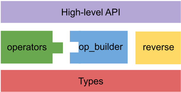
Fig. 8.4 shows the structure of the AD module, and we will introduce its components one by one, starting with the type definition.
type t =
  Owl_algodiff_generic.Make(Owl_algodiff_primal_ops.D).t =
    F of Owl.Algodiff.D.A.elt
  | Arr of Owl.Algodiff.D.A.arr
  | DF of Owl.Algodiff.D.t * Owl.Algodiff.D.t * int
  | DR of Owl.Algodiff.D.t * Owl.Algodiff.D.t ref * Owl.Algodiff.D.op *
      int ref * int * int ref
type adjoint =
    Owl.Algodiff.D.t ->
    Owl.Algodiff.D.t ref ->
    (Owl.Algodiff.D.t * Owl.Algodiff.D.t) list ->
    (Owl.Algodiff.D.t * Owl.Algodiff.D.t) list
type register = Owl.Algodiff.D.t list -> Owl.Algodiff.D.t list
type label = string * Owl.Algodiff.D.t list
type op =
    Owl.Algodiff.D.adjoint * Owl.Algodiff.D.register * Owl.Algodiff.D.label
There are several obvious differences to our earlier simple implementation. First,
besides DF and DR, the type definition also contains two other constructors, F and
Arr. F allows us to pack float numbers for scalar functions, whilst Arr can pack input
and output for the functions that handle ndarrays. You may also notice some extra
fields in the DF and DR constructors.
One important field is tag of type int, which is used to solve a particular
problem when calculating higher order derivatives with nested forward and backward
modes. This problem is referred to as perturbation confusion. Properly handling
perturbation confusion is important for any AD implementation; we only scratch the
surface of this problem here.
Consider: how should we compute the derivative of
i.e. a function that contains another derivative function. It initially seems straightforward: as so . Unfortunately, applying our previous simple implementation does not work.
# open Book_naive;;

# let diff f x =
      match x with
      | DF (_, _)    ->
        f x |> tangent
      | DR (_, _, _) ->
        let r = f x in
        reverse_push [(1., r)];
        !(adjoint x);;
val diff : (Book_naive.t -> t/8) -> Book_naive.t -> float = <fun>
# let f x =
      let g = diff (fun y -> add_ad x y) in
      mul_ad x (make_forward (g (make_forward 2. 1.)) 1.);;
val f : Book_naive.t -> t/8 = <fun>
# diff f (make_forward 2. 1.);;
- : float = 4.
The result is at point but we have previously calculated it should be at any point, so what has gone wrong?
Did you notice that x=DF(2,1)? The tangent value equals 1, which means that
.
Now if we continue to use this same x value in function g, whose variable is
y, the same x=DF(2,1) can be incorrectly translated by the AD engine as
.
Within the inner differentiation with respect to
,
must
have zero tangent for that differentiation level. Its outer tangent with respect to
must still be preserved; simply discarding that outer tangent would lose
information.
Tagging solves this nested derivative problem by distinguishing derivative calculations and their associated attached values using a unique tag for each application of the derivative operator. In that way, different inputs will be recognised properly by the AD engine. More details of this method are explained in [19].
Moving up we have the builder module that abstracts over the general process of
forward and reverse modes, and the operators module that contains the specific
calculation methods for each operation. Our simple implementation demonstrated
how to construct differentiation for unary and binary operations using two builder
modules, but of course there are many other operators with different types and so
Owl abstracts according to their number of input variables and output variables.
For example, the qr operation calculates QR decomposition of an input
matrix. This operation uses the SIPO (single-input-pair-output) builder
template.
Each operation in ops supplies rules for primal, tangent, and adjoint
computations, as in our simple example. The single-input, single-output builder
below separates the primal rule into ff_f for scalars and ff_arr for arrays, alongside
df and dr. However, in our simple example all the constants are either DF or DR and
so we must define both f_forward and f_reverse even though only the
definition of constants differs. But now that the float number is included
in the data type t, we can define just one computation function for both
modes:
open Algodiff.D;;
let f_forward x =
  let x0, x1 = x in
  let open Maths in
  let v2 = sin x0 in
  let v3 = mul x0 x1 in
  let v4 = add v2 v3 in
  let v5 = F 1. in
  let v6 = exp v4 in
  let v7 = F 1. in
  let v8 = add v5 v6 in
  div v7 v8;;
We next consider how to compute DR and F data types together, by considering
more cases in an operation than in our simple implementation which used just three
functions (ff, df, and dr). For ff a b, we must consider cases such as a is scalar
while b is an Ndarray. For df and dr, we must consider what happens if one input is
constant, either F or Arr. Finally, above these parts sits the high level APIs
introduced earlier.
8.7.2 Extending AD
A significant benefit of the module design described above is that it can
be easily extended by providing modules representing new functions. For
example, suppose that the AD system did not support the sine function,
, whose
derivative is .
Including this function is a simple matter of defining the necessary functions for
calculating primal, tangent, and adjoint values in a module, and applying the
relevant function from the Builder module – in this case, build_siso for building
“single input, single output” functions.
open Algodiff.D

module Sin = struct
  let label = "sin"
  let ff_f a = F A.Scalar.(sin a)
  let ff_arr a = Arr A.(sin a)
  let df _cp ap at = Maths.(at * cos ap)
  let dr a _cp ca = Maths.(!ca * cos (primal a))
end

let new_sin_ad = Builder.build_siso (module Sin : Builder.Siso);;
We can now use this function as if it were a native operation from the AD module. For example, we can use this new operator to build the calculation from our earlier example, and obtain the derivatives.
# let f x =
      let x1 = Mat.get x 0 0 in
      let x2 = Mat.get x 0 1 in
      Maths.(div (F 1.) (F 1. + exp (x1 * x2 + (new_sin_ad x1))));;
val f : Owl_algodiff.D.t -> Owl_algodiff.D.t = <fun>
# let x = Mat.ones 1 2;;
val x : Owl_algodiff.D.t = Owl_algodiff.D.Arr
   C0 C1
R0  1  1
# let _ = grad f x |> unpack_arr;;
- : Owl.Algodiff.D.A.arr =
          C0        C1
R0 -0.181974 -0.118142
8.7.3 Lazy Evaluation
The Builder module makes it convenient to add new operations, but where the
builder is called matters for efficiency. Imagine a large problem that consists of
thousands of operations, with one function occurring many times among those
operations.3
If the builder is called inside the operation’s body, it rebuilds the operator on each
call. Our earlier top-level binding already builds it once and reuses it. OCaml’s lazy
evaluation is another way to arrange for a computation to run at most once,
deferring it until it is forced.
OCaml provides the special expression syntax lazy expr, producing a deferred
computation of type ’a Lazy.t when expr has type ’a. It is not an ordinary
function that evaluates an argument before receiving it. The first call to
Stdlib.Lazy.force evaluates the deferred expression and caches its result.
Subsequent applications of Stdlib.Lazy.force will simply return the cached result
without further re-evaluation.
For example, imagine again that we need to add support for the sin operation.
The definition of sin remains the same:
open Algodiff.D

module Sin = struct
  let label = "sin"
  let ff_f a = F A.Scalar.(sin a)
  let ff_arr a = Arr A.(sin a)
  let df _cp ap at = Maths.(at * cos ap)
  let dr a _cp ca = Maths.(!ca * cos (primal a))
end;;
We can also place the builder call in a lazy expression and force it to obtain the implementation:
let _sin_ad = lazy (Builder.build_siso (module Sin : Builder.Siso));;
let new_sin_ad = Stdlib.Lazy.force _sin_ad;;
Here Stdlib.Lazy.force is called immediately when new_sin_ad is defined,
so construction is not delayed until the first call to the sine operator. The
builder still runs only once, just as with the earlier direct top-level binding. It
is the constructed operator that is reused, not the sine result for different
inputs.
8.8 Summary
In this chapter we have discussed algorithmic differentiation (AD) and its underlying theory, starting from the classic chain rule in differentiation, introducing the basic forward and reverse modes of AD, followed by a step-by-step illustration of how to implement a simple AD module. We finished with a more in-depth discussion of Owl’s AD module, and how to extend and optimise it. After finishing this chapter, you should have a solid understanding of both AD theory and its implementation.
Bibliography
- [1]
- Baydin AG, Pearlmutter BA, Radul AA, Siskind JM. Automatic differentiation in machine learning: a survey. Journal of Machine Learning Research. 2018;18(153):1–43.
- [2]
- Hecht-Nielsen R. Theory of the backpropagation neural network. Neural networks for perception 1992 Jan 1 (pp. 65-93). Academic Press.
- [3]
- Feynman RP, Leighton RB, Sands M. The Feynman Lectures on
Physics. Vol. II, Chapter 2: Differential Calculus of Vector Fields.
California Institute of Technology, online edition. Available from:
https://www.feynmanlectures.caltech.edu/II_02.html. - [4]
- Courant R, John F. Introduction to calculus and analysis I. Springer Science & Business Media; 2012 Dec 6.
- [5]
- Atkinson KE. An introduction to numerical analysis. John wiley & sons; 2008.
- [6]
- Fischer H, Warsitz H. Complexity of derivatives generated by symbolic differentiation. In Computer Algebra in Scientific Computing 2000 (pp. 129-144). Springer, Berlin, Heidelberg.
- [7]
- Margossian CC. A review of automatic differentiation and its efficient implementation. Wiley interdisciplinary reviews: data mining and knowledge discovery. 2019;9(4):e1305.
- [8]
- Paszke A, Gross S, Chintala S, Chanan G, Yang E, DeVito Z, Lin Z, Desmaison A, Antiga L, Lerer A. Automatic differentiation in PyTorch. NIPS 2017 Workshop on Autodiff; 2017.
- [9]
- Naumann U. The art of differentiating computer programs: an introduction to algorithmic differentiation. Society for Industrial and Applied Mathematics; 2012.
- [10]
- Griewank A. On automatic differentiation. In: Iri M, Tanabe K, editors. Mathematical Programming: Recent Developments and Applications. Kluwer Academic Publishers; 1989. pp. 83–108.
- [11]
- Python AD [Internet]. Welcome to the ad package - ad Python
package 1.3.2 documentation. [cited 2021 Dec 5]. Available from:
https://pythonhosted.org/ad/. - [12]
- Juliadiff [Internet]. JuliaDiff. [cited 2021 Dec 5]. Available from:
https://juliadiff.org/. - [13]
- MathWorks. dlgradient: Compute gradients for
custom training loops using automatic differentiation.
MATLAB documentation [Internet]. Available from:
https://www.mathworks.com/help/deeplearning/ref/dlarray.dlgradient.html. - [14]
- Vishwanathan SV, Schraudolph NN, Schmidt MW, Murphy KP. Accelerated training of conditional random fields with stochastic gradient methods. Proceedings of the 23rd international conference on Machine learning 2006 Jun 25 (pp. 969-976).
- [15]
- Homescu C. Adjoints and automatic (algorithmic) differentiation in computational finance. Available at SSRN 1828503. 2011 Sep 12.
- [16]
- Ruder S. An overview of gradient descent optimization algorithms. arXiv preprint arXiv:1609.04747. 2016 Sep 15.
- [17]
- Curry HB. The method of steepest descent for non-linear minimization problems. Quarterly of Applied Mathematics. 1944. 2(3):258-61.
- [18]
- Hartman-Grobman theorem [Internet]. Wikipedia. Wikimedia Foundation;
2021 [cited 2021 Dec 5]. Available from:
https://en.wikipedia.org/wiki/Hartman-Grobman_theorem. - [19]
- Siskind JM, Pearlmutter BA. Perturbation confusion and referential
transparency: Correct functional implementation of forward-mode
AD. IFL 2005: 17th International Workshop on Implementation
and Application of Functional Languages; 2005. Available from:
https://mural.maynoothuniversity.ie/id/eprint/566/.