CHAPTER 12
Reinforcement Learning
A prediction tells us what may happen; a decision changes what happens next. Reinforcement learning studies how an agent learns to make decisions through interaction with an environment. Using owl-rllib, we move from finite Markov decision processes and planning to learning values and policies with neural networks. We then apply these ideas to a small language model, LunarLander and VizDoom.
In the previous chapter, a neural network learned from examples whose desired outputs were already available. Consider instead a program that must land a spacecraft. We can observe its position and velocity, and we can fire its engines, but there is no table telling us the best action for every situation. Moreover, a useful action may not give an immediate benefit: slowing the descent now may prevent a crash much later. In reinforcement learning, the agent learns through actions and their consequences, seeking a large cumulative reward.
12.1 Markov Decision Processes
Let us begin with a world small enough to describe completely. An agent occupies one cell of a grid. It can move up, right, down or left. A move outside the grid leaves it where it is. Two opposite corners are terminal cells: arriving at either one ends the episode. Each move, including a move into a terminal cell, gives reward . The agent should therefore find a short route to a corner.
A Markov decision process (MDP) describes such a world using a set of states , actions , and a distribution over the next state and reward. The Markov assumption says that the current state and action contain the information needed for this distribution; the complete history is unnecessary. In the grid, the cell is a state and the transition is deterministic. In a physical system, position alone may be insufficient: velocity also affects what happens next. This distinction matters when choosing an observation for a learning algorithm.
The agent’s rule for acting is its policy. A stochastic policy gives a probability for each action at state . A deterministic policy chooses one action. An episode produces a sequence
We use for the reward received after action . The return from time is
| (12.1) |
For a continuing task the sum extends indefinitely; bounded rewards and make it finite. The discount factor controls the relative importance of later rewards. In an episodic task, is also useful when the expected return exists. For our grid with unit step cost, the undiscounted return is minus the number of moves before termination.
The state-value function is the expected return under a given policy:
It is a property of both the world and the policy. The same cell can have a low value under a wandering policy and a high value under a policy that heads straight towards the nearest corner. Separating the first reward from the remaining return gives the Bellman equation:
| (12.2) |
Here the value after a terminal transition is zero. Equivalently, an implementation can multiply the continuation value by a flag that is zero at termination.
The first example constructs the grid and evaluates a policy that gives each direction probability :
let grid = Gridworld.sutton_4x4 ()
let mdp = grid.mdp
let uniform = Array.make_matrix mdp.n_states mdp.n_actions 0.25
let values = Dp.policy_evaluation ~gamma:1. mdp uniform
The library represents the finite model as a transition table. For each state and action, its entries contain a probability, a next state, a reward and a terminal flag. This representation also allows several possible outcomes of one action. The complete program checks that probabilities sum to one and that the computed values satisfy Eq. 12.2:
G . . .
. . . .
. . . .
. . . G
      G  -14.0  -20.0  -22.0
  -14.0  -18.0  -20.0  -20.0
  -20.0  -20.0  -18.0  -14.0
  -22.0  -20.0  -14.0      G
Bellman residual below 1e-8 in all 16 states.
The value next to a corner is , even though the corner can be reached in a single move. There is no contradiction: the policy chooses randomly rather than deliberately taking that move. The values describe its expected wandering time. This grid is the small policy-evaluation example in Sutton and Barto [1]; the progression from finite models to sampled updates also follows the CS188 treatment [2].
An action-value function additionally conditions on the first action:
Thus . A value answers how good it is to be in a state; an action value answers how good it is to take a particular action there and then follow the policy.
12.2 Planning with a Known Model
When the transition table is available, we can calculate values without sampling episodes. Policy evaluation repeatedly applies the right-hand side of Eq. 12.2. With , this update is a contraction in the maximum norm, so successive sweeps converge to the unique fixed point. For , convergence requires additional conditions, such as the proper episodic policy used in our grid.
The same equation can be written in matrix form. Let be the transition matrix after averaging over actions and omitting continuation at terminal transitions, and let be the expected immediate reward vector. Then
This connects policy evaluation to the linear systems in Chap. 4. Iterative sweeps are attractive when the model is sparse or large, because they need not construct an inverse.
12.2.1 Improving a Policy
Suppose we have evaluated a policy. We can ask whether taking another first action would give a better expected return, while keeping the old policy thereafter. A greedy improvement chooses
Policy iteration alternates evaluation and improvement until the policy is stable. Value iteration instead applies a maximum at every value update:
| (12.3) |
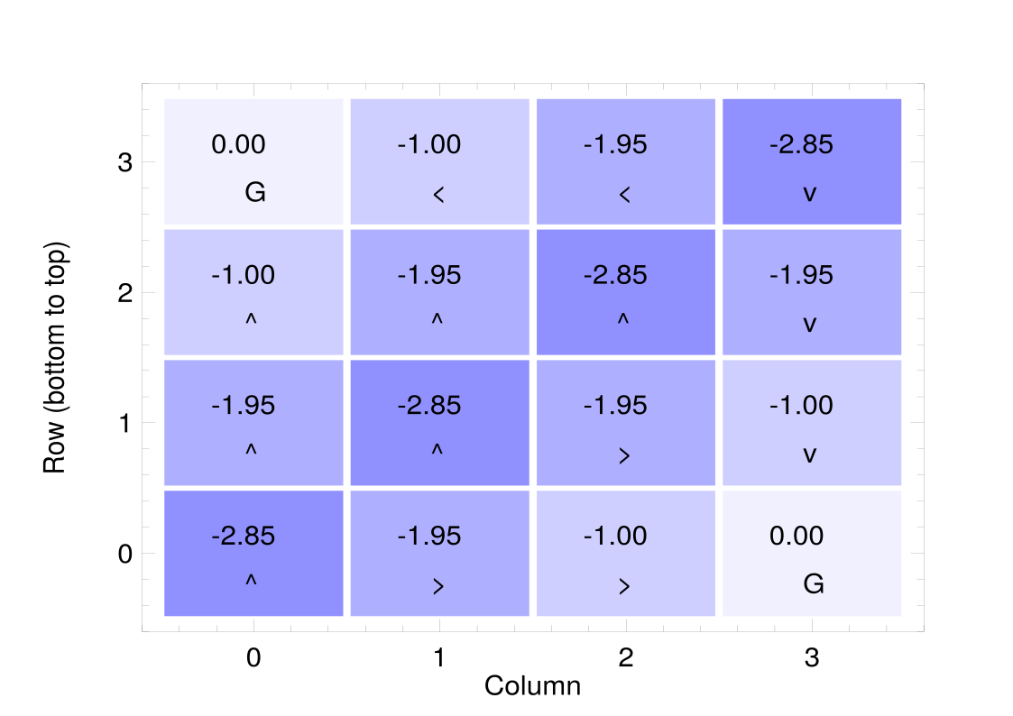
After convergence, a greedy policy is optimal for the finite discounted MDP. Ties can give several optimal policies, so matching values is a more useful implementation check than requiring identical action arrays.
The following code compares both algorithms on the grid, now using :
  let grid = Gridworld.sutton_4x4 () in
  let pi, v = Dp.value_iteration ~gamma:0.95 grid.mdp in
  let _, vp = Dp.policy_iteration ~gamma:0.95 grid.mdp in
  Array.iter2 (fun a b -> assert (abs_float (a-.b) < 1e-7)) v vp;
  Gridworld.print_values grid v;
  Gridworld.print_policy grid pi;
Figure 12.1 shows the resulting values and one optimal action in each non-terminal cell.
12.2.2 Planning on Slippery Ice
In FrozenLake, the agent must cross a frozen surface while avoiding holes. The goal gives reward one, and other transitions give zero. On slippery ice, the intended direction and the two perpendicular directions each occur with probability . Switching off slipping makes the transitions deterministic. The algorithm remains the same; only the model changes:
  List.iter (fun slippery ->
    let lake = Frozen_lake.make ~slippery () in
    let _, optimal = Dp.value_iteration ~gamma:0.95 lake in
    let random = Dp.policy_evaluation ~gamma:0.95 lake
        (Array.make_matrix 16 4 0.25) in
    assert (optimal.(0) >= random.(0));
    Printf.printf "Slippery=%b: random value %.4f; optimal %.4f\n"
      slippery random.(0) optimal.(0)) [false; true]
At , our start-state optimal value is about without slipping and with slipping. These are discounted expected rewards, not raw probabilities of success. A successful path that takes longer receives a smaller discounted return. With , in a setting where the only nonzero reward is one on reaching the goal, the expected return can instead be interpreted as the probability of eventually reaching it.
A policy for the slippery lake may point towards a boundary. A blocked movement leaves the agent in place, which can be safer than allowing a sideways slip into a hole. Planning accounts for the outcomes of an action, rather than assuming that its name describes what will certainly happen.
12.3 Learning without a Model
A complete transition table is convenient, but often unavailable. We may only be
able to reset the environment and take an action. The Env.of_mdp adapter gives
exactly this interface for a finite model. It lets us test learning algorithms in a world
whose exact solution we can still calculate separately.
12.3.1 Monte Carlo and Temporal-Difference Prediction
Monte Carlo prediction estimates by averaging observed returns after visits to . It needs complete episodes, but does not need transition probabilities. An incremental mean has the familiar form
where gives an arithmetic average after returns for state . One can use the first visit in each episode or every visit, provided that the counting convention matches the estimator.
Temporal-difference learning replaces the full return by a one-step estimate:
| (12.4) |
This is TD(0). It can update immediately after a transition. Using the current estimate of a future value is called bootstrapping. Monte Carlo waits for the observed outcome; TD uses a prediction to update another prediction. At true termination, the continuation term is zero.
Our example estimates the value of a uniform random policy on FrozenLake using both methods:
  let lake = Frozen_lake.make () in
  let gamma = 0.95 in
  let exact = Dp.policy_evaluation ~gamma lake (Array.make_matrix 16 4 0.25) in
  let env = Env.of_mdp ~rng lake in
  let policy _ = Random.State.int rng 4 in
  (* Monte Carlo waits for the end of the episode and averages the returns. *)
  let mc = Tabular.mc_prediction ~gamma ~episodes:20_000 ~policy env in
  (* TD(0) updates after every step, using its own estimate of the next state. *)
  let td = Tabular.td0_prediction ~gamma ~alpha:0.02 ~episodes:20_000 ~policy env in
The complete program prints the exact, Monte Carlo and TD estimates for selected states. After 20,000 episodes, the start-state estimates are approximately , and , respectively. TD uses a fixed step size here, so recent observations retain more influence than in an arithmetic mean.
12.3.2 Q-learning, SARSA and Exploration
For control we must also improve the policy. An -greedy rule chooses a uniformly random action with probability , and otherwise takes a greedy action. A greedy action can also be selected by the random branch. This simple mechanism balances exploration, which obtains information, against exploitation, which uses the current estimates.
Two control updates differ in the action used for bootstrapping. Q-learning uses the best estimated next action:
| (12.5) |
SARSA uses the next action actually sampled from the behaviour policy:
| (12.6) |
SARSA is on-policy: its target includes the behaviour policy’s future exploration. Q-learning is off-policy: its greedy target differs from the exploratory policy collecting the data. In a finite discounted MDP, tabular Q-learning has convergence guarantees under sufficient visits and suitable decreasing step sizes.
CliffWalking makes the distinction visible. The start and goal lie at opposite ends of the bottom row, with a cliff between them. Ordinary steps cost one; stepping into the cliff costs 100 and returns the agent to the start. We train both methods with :
  let cliff = Cliff_walking.make () in
  let run algorithm =
    let env = Env.of_mdp ~rng cliff in
    algorithm rng ~gamma:1. ~alpha:0.5 ~epsilon:0.1 ~episodes:500 env
  in
  let q_sarsa, r_sarsa = run Tabular.sarsa in
  let q_qlearn, r_qlearn = run Tabular.q_learning in
Figure 12.2 tracks the returns while both agents continue to explore.
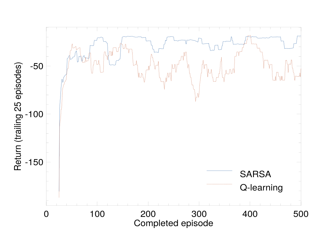
In this run, the greedy policy learned by Q-learning follows the row immediately above the cliff. SARSA takes a longer route further away. The Q-learning target assumes greedy future actions, while SARSA includes the possibility of a later exploratory step towards the cliff. Consequently, the shorter greedy path need not have the better return while exploration remains active. The mean returns over the final 100 training episodes are about for SARSA and for Q-learning. This is the distinction illustrated by Sutton and Barto’s Example 6.6 [1].
The same program applies Q-learning to Taxi, which has 500 states encoding the taxi location, passenger location and destination. No new update rule is needed. What grows is the table, and the amount of experience required to fill it. This limitation becomes much more serious when observations are continuous.
12.4 From Tables to Function Approximation
A CartPole observation contains position, velocity, angle and angular velocity. Even a modest discretisation can create a large state table, and neighbouring observations should usually share information. A function approximator gives us this sharing.
12.4.1 Linear Features
For a feature vector , a linear action value has the form
In a semi-gradient SARSA update, we form the target and update
The word semi-gradient means that the target is held fixed when taking the derivative, even though it also contains current weights.
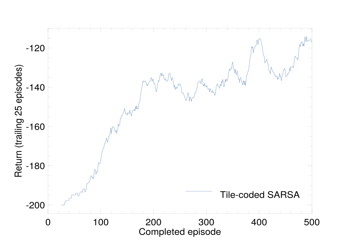
MountainCar is a useful example. The car cannot drive straight up the steep hill with its weak engine; it must first build momentum. The observation contains position and velocity. We represent them with eight overlapping grids, called tile coding. An observation activates one tile in each grid:
let features obs =
  let x = (A.get obs [| 0 |] +. 1.2) /. 1.8 *. 8.
  and v = (A.get obs [| 1 |] +. 0.07) /. 0.14 *. 8. in
  Array.init 8 (fun t ->
    let ix = min 8 (max 0 (int_of_float (floor (x +. float_of_int t /. 8.)))) in
    let iv = min 8 (max 0 (int_of_float (floor (v +. float_of_int ((3 * t) mod 8) /. 8.)))) in
    t * 81 + ix * 9 + iv)
The feature vector has entries, but only eight are nonzero. The program returns their indices instead of constructing a dense vector. Learning then touches only the corresponding weights:
  let env = Mountain_car.make ~rng:rngs.env () in
  let weights, returns = Linear.S.train ~features ~n_features:(8*81)
      ~gamma:1. ~alpha:0.3 ~epsilon:0.01 ~episodes:500
      ~rng:rngs.action env in
In Fig. 12.3, returns become less negative as the car learns to reach the goal sooner.
The library divides the supplied step size by the number of active features. With
alpha=0.3, each active feature therefore receives one eighth of the nominal step
size.
12.4.2 Deep Q-networks
A neural network can learn its own nonlinear representation. For a discrete action space, its output has one component per action. We train this network towards the same kind of target as in Eq. 12.5. However, successive transitions are correlated, and changing the network also changes the bootstrap target.
A deep Q-network (DQN) uses two mechanisms to address these difficulties [3]. First, an experience replay buffer stores transitions and draws random minibatches from them. Second, a separate target network, with parameters , supplies the continuation values. It is held fixed between periodic copies from the online network. A target for transition is
where indicates true termination. The implementation used here minimises the mean squared error
The target is treated as a constant during this update. Replay makes old transitions useful for several updates, while the target network slows changes in the regression target.
The CartPole example uses a two-hidden-layer network and an explicit switch for the target network:
let train target_network =
  let rngs = Rng.create 42 in
  let network = N.mlp ~seed:rngs.network_seed ~shape:[|4|]
      ~hidden:[64;64] ~outputs:2 in
  let config = { Dqn.S.default with target_network } in
  let returns = Dqn.S.train ~config ~steps:total_steps ~rngs ~network
      (Cartpole.make ~rng:rngs.env ()) in
Figure 12.4 compares the training returns with and without the separate target network.
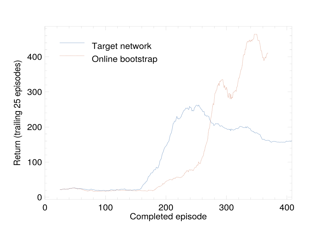
Target network=true: greedy evaluation 141.8
Target network=false: greedy evaluation 492.4
Target network: 408 episodes; last 25 mean 160.68
Online bootstrap: 369 episodes; last 25 mean 410.48
In this run, removing the target network improved the final greedy evaluation return from to . The separate network keeps the bootstrap target fixed between copies; here that slower-moving target did not yield a higher return. We use the same target-network mechanism again in the pixel-based VizDoom case study (Sect. 12.9).
12.4.3 Termination and Time Limits
An episode can end because the task has finished, or because a wrapper has
stopped collecting experience. The environment interface separates terminated from
truncated. For a true terminal transition, no future reward remains. At an external
time limit in a continuing task, a value estimate can still supply a continuation. DQN
therefore masks bootstrapping with terminated, while either flag causes a reset
before the next episode.
The task definition decides which interpretation is appropriate. If a fixed deadline is part of the task itself, the remaining time may need to be included in the state, and reaching it is terminal.
12.5 Policy Gradients
So far we have obtained a policy indirectly, by choosing actions with large estimated values. We can instead parameterise the policy itself. For discrete actions, a neural network produces logits and a softmax turns them into action probabilities. For a continuous action, a network can produce the parameters of a distribution from which an action is sampled.
The pole is tipping, and the cart must move. Suppose the policy assigns a probability of to pushing left and to pushing right. Sampling can still choose left. The agent records that choice, takes the action, and watches what happens next:
cart and pole
Policy
left: ; right:
Sample
left
A larger return gives this sample more weight in the update. The network can then make left more likely when it sees that state again. But how much of the episode’s success should count towards this particular push?
Imagine a treasure game. Two paths meet at the same junction. On one path the player has already earned eight points; on the other, the player has lost four. From the junction onwards the situation is identical. In both episodes the player turns right, earns nothing immediately, then falls into a pit costing three points and ending the game. With no discounting, the records are:
| Earlier | Turn right | Pit | Total | From turn | |
| Episode A | |||||
| Episode B | |||||
Using the whole episode’s return would give the same turn a positive training weight in A and a negative one in B. The difference comes entirely from events before the junction. Using only rewards from the turn onwards gives both samples the same weight, . This is the reward-to-go . With , the immediate zero and the following penalty instead give . The discount changes how much the later penalty counts.
We can now connect this bookkeeping to a gradient. Let denote a sampled trajectory and let . Its probability factors into the initial-state distribution , policy choices and environment transitions:
For a fixed trajectory, changing the policy parameters changes the probabilities of the recorded choices. The environment factors stay fixed. Taking the logarithm turns the product into a sum, so its gradient is the sum of the individual action log-probability gradients. The identity expresses the return gradient as an average of these gradients weighted by the episode return.
As the treasure example suggests, earlier rewards add noise to an action’s weight. Their contributions to the expected policy gradient are zero, so we can remove them without changing that expectation. Keeping the reward-to-go gives
| (12.7) |
The three factors inside the sum have distinct jobs: locates the action in the discounted objective, the log-probability gradient tells us how to change its probability, and weights that gradient by the rewards observed from this action onwards. This is the basis of REINFORCE [4]. We differentiate the policy; the simulator supplies experience.
Return to the CartPole choice. For a hand calculation, set and suppose that three rewards of remain from the sampled left push to termination. Its return is three. In the previous chapter, a labelled image told the classifier which output to favour. Here we have a recorded choice, left, and an observed return that weights its contribution. The corresponding loss term is . At probability it is about ; at probability it is about . Minimising this term favours a higher probability of left. The other sampled choices contribute their own terms to the update.
For a batch of episodes sampled under the current policy, we collect those terms into the loss
| (12.8) |
The sampled states, actions and returns are held fixed during differentiation. The minus sign turns gradient ascent on return into gradient descent on this loss. The outer factor accounts for the time of the action in ; discounts later rewards relative to that action.
The training loop collects episodes, computes returns backwards, and updates the network with this loss. In the three-step CartPole tail, the undiscounted returns are one for the last action, two for the preceding action, and three for the first. The same backward calculation uses when discounting is enabled. After updating, the agent collects fresh episodes under its new policy. This dependence on the sampling policy will motivate PPO’s probability ratio when we reuse data for several updates.
12.5.1 Subtracting a Baseline
Three more points sound like good news. But suppose that, from this CartPole state, the policy usually earns about twenty more points. Surviving for only three steps is then a disappointing result. A continuation lasting thirty steps would be much better. The raw returns give both sampled choices positive weights, three and thirty, even though one outcome falls well below the usual performance.
A state-dependent baseline supplies the comparison. Using twenty in this hand calculation changes the weights to and . With a weight of , this sample pushes down the probability of its action. With , it pushes it up. In the loss, we simply replace by . Thus the baseline changes what counts as a favourable outcome at each state.
This subtraction preserves the expected policy gradient when the baseline is independent of the sampled action. At a fixed state, the action probabilities sum to one. Differentiating that sum gives zero, so the policy-weighted average of their log-probability gradients is zero too; multiplying by a common still gives zero. The baseline changes the variation between sample updates. A separate value network can learn this baseline by predicting returns. Its predictions are held fixed while differentiating the policy loss.
To measure the effect of subtracting a baseline, the baseline-variance example
freezes a trained policy and its critic. It collects 64 further trajectories and computes
two gradient estimates on each same trajectory: one using the observed returns, the
other subtracting the critic. Both use the same finite-trajectory Monte Carlo
targets and discount weights. We measure the sum of the per-parameter
sample variances, or the trace of the gradient covariance matrix:
Frozen policy, 64 shared held-out trajectories:
Gradient covariance trace: raw 93548.3; baseline 85944.4
Variance ratio 0.919; critic MSE 2013.83
The ratio is : subtracting this critic reduces the measured variance by about . The policy stays fixed throughout this comparison.
We also train CartPole policies with and without the value network:
let train use_baseline =
  let rngs = Rng.create 0 in
  let policy = N.mlp ~seed:rngs.network_seed ~shape:[|4|]
      ~hidden:[64] ~outputs:2 in
  let critic = if use_baseline then
      Some (N.mlp ~seed:(rngs.network_seed+1) ~shape:[|4|]
              ~hidden:[64] ~outputs:1) else None in
  Reinforce.S.train ?baseline:critic ~episodes ~rng:rngs.action
    ~policy (Cartpole.make ~rng:rngs.env ())
Figure 12.5 shows their training returns. Over the final 25 episodes, the means are without the baseline and with it. Here the value network also supplies the bootstrap value at time limits, while the version without it uses the finite observed return. These training runs therefore compare both baseline use and truncation handling; the frozen-policy measurement above measures the variance change directly.
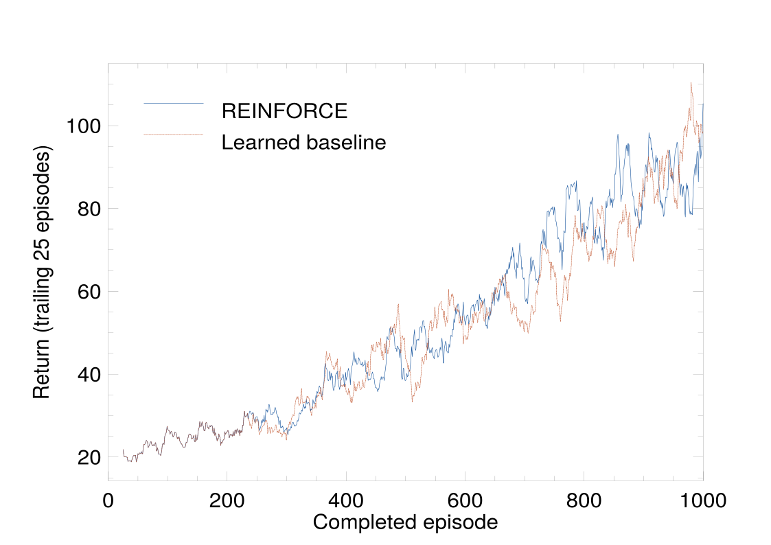
We will see in the language-model example how a different baseline and task can increase gradient variance.
12.6 Actor–Critic Methods
A value network can do more than supply a baseline for complete Monte Carlo returns. It can help estimate returns before an episode finishes. In an actor–critic method, the actor represents the policy and the critic estimates a value. The advantage
measures the improvement over the average action under the policy. Replacing a raw return by an advantage estimate gives the actor a more local learning signal.
12.6.1 Advantage Estimation
The one-step TD residual is one possible advantage estimate. Generalised advantage estimation (GAE) combines several residuals [5]:
| (12.9) |
The sum stops at the rollout or episode boundary. At , it uses one residual. Larger includes more observed rewards and relies less on short-range bootstrapping. A training target for the critic is , with the old values held fixed.
Implementation details at boundaries matter. The TD residual bootstraps at an external truncation, but the backward GAE recursion must stop there: the next episode begins from a different initial state. At a true termination, both the bootstrap and the recursion stop. The library stores the final observation of a transition separately from any observation produced by a later reset.
12.6.2 A2C and PPO
Synchronous advantage actor–critic (A2C) collects a short rollout from several environments, then updates actor and critic once. An entropy term can encourage exploration. It is on-policy: after an update, the next rollout is collected under the updated policy. In owl-rllib the vector environment steps its environments in sequence and batches their observations for the network.
Proximal policy optimisation (PPO) reuses each rollout for several epochs [6]. To account for a policy changing after data collection, define the probability ratio
The clipped objective averages
| (12.10) |
For a positive advantage, raising the probability ratio above no longer improves the objective term. For a negative advantage, lowering the ratio below no longer improves it. The minimum makes clipping depend on the sign of the advantage. The clip acts on the objective; the optimiser can still move probability ratios beyond the clipping interval. The Kullback–Leibler (KL) divergence measures how the updated action distribution differs from the old one.
The actor minimises the negative of Eq. 12.10, with any entropy term added according to its sign convention. The critic minimises a value-regression loss. Recorded old log probabilities and advantage estimates remain fixed while a rollout is reused. Once its epochs are complete, fresh experience is collected.
The following example compares the library’s default A2C and PPO configurations on CartPole:
let train a2c =
  let rngs = Rng.create 0 in
  let policy = N.mlp ~seed:rngs.network_seed ~shape:[|4|]
      ~hidden:[64;64] ~outputs:2 in
  let critic = N.mlp ~seed:(rngs.network_seed+1) ~shape:[|4|]
      ~hidden:[64;64] ~outputs:1 in
  let env = Vec_env.create (Array.init 8 (fun i ->
    Cartpole.make ~rng:(Random.State.make [|0;0;i|]) ())) in
  if a2c then
    A2c.S.train ~updates:(total_steps / (8*A2c.S.default.horizon))
      ~rngs ~policy ~critic ~distribution:Policy.S.categorical env
  else
    Ppo.S.train ~updates:(total_steps / (8*Ppo.S.default.horizon))
      ~rngs ~policy ~critic ~distribution:Policy.S.categorical env
Figure 12.6 shows how the two configurations learn over completed episodes.
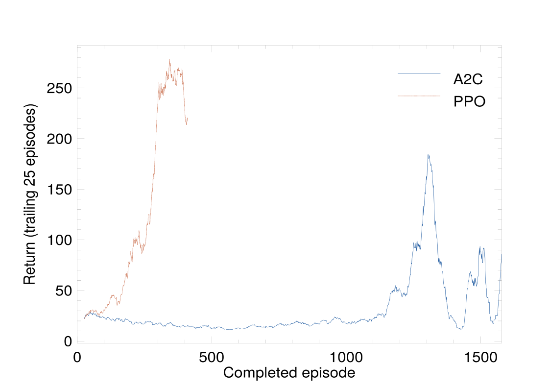
A2C collects five steps per environment and makes one update per rollout. PPO collects 128 steps per environment and makes four passes over each rollout in minibatches of 64. With the same 51,200-step budget, their final 25-episode mean returns are and , respectively. The horizontal axis counts completed episodes: longer-lived policies complete fewer episodes within that budget.
For continuous control, the policy can output a Gaussian mean and log standard deviation. For example, Pendulum has one bounded torque action. The same PPO training interface accepts a Gaussian distribution and an ndarray action instead of an integer. The environment and the algorithm agree on observation and action types, while the distribution supplies sampling, log probabilities and entropy:
  let policy = N.mlp ~seed:rngs.network_seed ~shape:[|3|]
      ~hidden:[64;64] ~outputs:2 in
  let critic = N.mlp ~seed:(rngs.network_seed+1) ~shape:[|3|]
      ~hidden:[64;64] ~outputs:1 in
  let distribution = Policy.S.gaussian ~low:[|-2.|] ~high:[|2.|] in
  let env = Array.init 8 (fun _ ->
    let e = Pendulum.make ~rng:(Random.State.make [|Random.State.bits rngs.env|]) () in
    { e with Ndenv.step = (fun a -> let st = e.step a in
        { st with reward = st.reward *. 0.1 }) }) |> Vec_env.create in
  let returns = Ppo.S.train ~updates:100 ~rngs ~policy ~critic ~distribution env in
The two policy outputs are the mean and log standard deviation for one torque. The policy samples an unconstrained Gaussian action. The adapter keeps that sample for the log-probability calculation, but clips the action sent to Pendulum to . Training scales rewards by ; evaluation reports the original reward. After 102,400 environment steps, the mean-action policy has a mean return of over 20 evaluation episodes.
12.7 Reinforcement Learning for Language Models
The same ideas apply when an action is a token. A prompt is the initial state, the growing prefix is the state, and the next token is the action. Appending a token gives a deterministic transition. A reward can be assigned to the completed answer. This is a useful bridge from ordinary policy gradients to language-model training, as developed in Wolfe’s overview [7].
We will use a small autoregressive model on two-digit addition. A prompt such as
27+48= should be followed by the tokens for 75 and an end-of-sequence token. The
vocabulary has 14 tokens: ten digits, the two operators, an end marker and a padding
marker. The model reads the last nine tokens, one-hot encodes them, and
passes them through two hidden layers of width 128. It demonstrates the
training procedure without requiring a large pretrained model or a transformer
implementation.
12.7.1 A Supervised Starting Point
There are 8,100 ordered pairs of operands from 10 to 99. A fixed split assigns 6,480 to training and 1,620 to testing. We first use supervised fine-tuning (SFT), training on correct completions with a cross-entropy loss. Teacher forcing supplies the correct previous tokens while predicting each next answer token. We stop after 500 steps so that there is room for reinforcement learning to improve the policy:
  let train, test = Lm_task.split ~seed:0 () in
  let policy = R.create ~seed:1 () in
  R.sft ~steps:sft_steps ~rng:(Random.State.make [|1|]) policy train;
  let reference = R.Graph.copy policy in
The copied network is a frozen reference. It must not change when the policy is updated.
A program can verify an addition answer exactly. Our outcome reward is one for the complete correct answer, including its end marker, and zero otherwise. This is an example of reinforcement learning with verifiable rewards. A learned reward model is not needed for this task. For a completion and prompt , the policy probability factorises as
REINFORCE could multiply the sum of these token log probabilities by the final reward. The supervised phase instead raises the probability of a supplied correct answer. RL samples answers from the current policy and changes their probabilities using the verifier’s feedback.
12.7.2 Group-relative Policy Optimisation
Group-relative policy optimisation (GRPO) estimates a relative quality from several answers to the same prompt, avoiding a separately trained critic [8]. For rewards in one group, our implementation computes
It uses the sample standard deviation. Each token in completion receives the same group-relative advantage. A small example makes this calculation explicit:
  let rewards = [|0.;1.;0.;1.; 0.;0.;0.;0.|] in
  let advantages = Lm_rl.grpo ~group_size:4 rewards in
  Array.iter (Printf.printf "%+.3f ") advantages;
  print_newline ();
  assert (Array.for_all ((=) 0.) (Array.sub advantages 4 4));
The first group produces approximately ; the second produces . An all-correct group also has zero relative advantages. Such a group provides no reward-surrogate gradient, although a separate regularisation term can still contribute.
GRPO uses a clipped token-probability ratio like Eq. 12.10. There are three policies to distinguish: the current policy being updated, the old policy that sampled the current group, and the frozen reference copied after SFT. The old policy changes between sampling iterations; the reference stays fixed throughout RL training.
The default configuration uses 64 prompts, eight completions per prompt, four updates on each sampled batch, clipping at , and a reference penalty with coefficient . It averages token losses within each completion and then averages over completions. Averaging within completions gives each answer equal weight regardless of its length.
The reference penalty discourages the policy from drifting too far from the model obtained by SFT. For a sampled token, it uses
where is the prefix. At a fixed prefix, the expected value of under the current policy equals its forward KL divergence to the reference. On later updates to the same batch, the penalty is averaged over tokens drawn from the old sampling policy. We differentiate this penalty along with the reward surrogate.
We train with these settings:
  let stats = R.train_grpo ~reference ~iterations ~rngs:(Rng.create 7)
      ~problems:train policy ~report:(fun i _ ->
        if i mod 50 = 0 then evaluate i) in
Figure 12.7 follows sampled and greedy test accuracy through the RL updates.
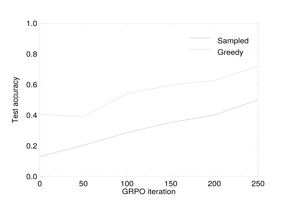
In this run, sampled accuracy increases from after SFT to , while greedy accuracy increases from to . Greedy decoding can be much better than sampling when a correct token has the largest probability but substantial probability remains on alternatives.
12.7.3 Two Useful Failure Cases
First, the end marker is part of the answer. If the model reaches the token limit without producing the end marker, the answer has failed and the episode ends. An earlier token-environment experiment used per-token process rewards and a critic. It treated this limit as an external truncation and used the critic to estimate further rewards. After 32,768 episodes, both sampled and greedy test accuracy were ; treating the limit as termination gave and , respectively [11]. The faulty policy learned to omit the end marker. This is the task-definition issue from Sect. 12.4.3 in another form: the meaning of the boundary must match the reward.
Second, subtracting a baseline does not automatically reduce variance. In a separate addition experiment after 1,500 SFT steps, subtracting the batch mean reward increased the gradient variance to times the value without a baseline. The comparison used the same frozen policy and 32 shared batches of 512 completions [11]. For wrong answers, the gradient of the sequence log probability was much larger in magnitude than for correct answers. Their zero reward gives these gradients zero weight. Subtracting a positive baseline gives them negative weights, so they contribute to the update. In this experiment, those contributions increased the variance. For a constant baseline and sequence score , the variance-minimising value is
which need not equal the mean reward. The owl-rllib program
examples/llm/b1_formulation.ml reproduces the termination comparison with the
options --process, --critic and --truncate. The baseline comparison is in
examples/llm/b2_reinforce.ml. The companion notes record the original
experiment versions and results [11].
12.8 Case Study: Landing a Spacecraft
Gymnasium’s LunarLander provides eight observations: horizontal and vertical position, the corresponding velocities, angle, angular velocity, and two leg-contact indicators. The discrete actions do nothing, fire one of the side engines, or fire the main engine. The reward combines progress towards a controlled landing with penalties for engine use and a terminal outcome [9].
These figures use LunarLander-v2 from Gymnasium 0.29.1. The simulator runs in
a Python child process, while the policy, critic and optimiser run in OCaml. We
create a policy with four outputs and a critic with one:
  let policy = N.mlp ~seed:rngs.network_seed
      ~shape:[|8|] ~hidden:[64; 64] ~outputs:4 in
  let critic = N.mlp ~seed:(rngs.network_seed + 1)
      ~shape:[|8|] ~hidden:[64; 64] ~outputs:1 in
  let make rng = Gym.S.discrete
      ~seed:(Random.State.bits rng) "LunarLander-v2" in
Sixteen environments contribute 1,024 transitions each to a rollout. We use a longer reward horizon than in CartPole by choosing , together with and an entropy coefficient of :
let total_steps = 16_384  (* Figure: 1_000_000 steps *)
let seed = 0
let config = { Ppo.S.default with
  horizon = 1024; gamma = 0.999; lambda = 0.98;
  entropy_coef = 0.01 }
The default budget performs one complete rollout and its updates. To reproduce the
longer experiment, change total_steps to 1_000_000, or pass --steps
1000000 to the compiled program. The program rounds down to complete
rollouts, so the figure uses 999,424 environment steps. Add --frames to
export evaluation frames and evaluate 20 episodes before and after training.
  let env = Vec_env.create (Array.init 16 (fun _ -> make rngs.env)) in
  let curve = Ppo.S.train ~config ~updates ~rngs ~policy ~critic
      ~distribution:Policy.S.categorical env in
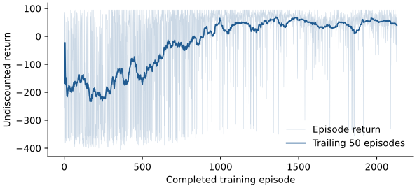
Figure 12.8 shows the exploratory training returns as the policy learns to land.
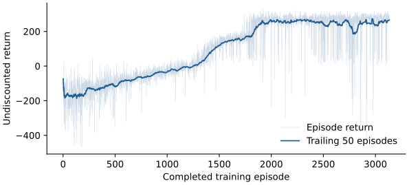
Across the same 20 held-out evaluation episodes, mean return rose from before training to afterwards. Evaluation selects the most probable action at each step; the training curve includes exploratory actions. The images in Fig. 12.9 show the first evaluation episode, using the same environment seed before and after training.
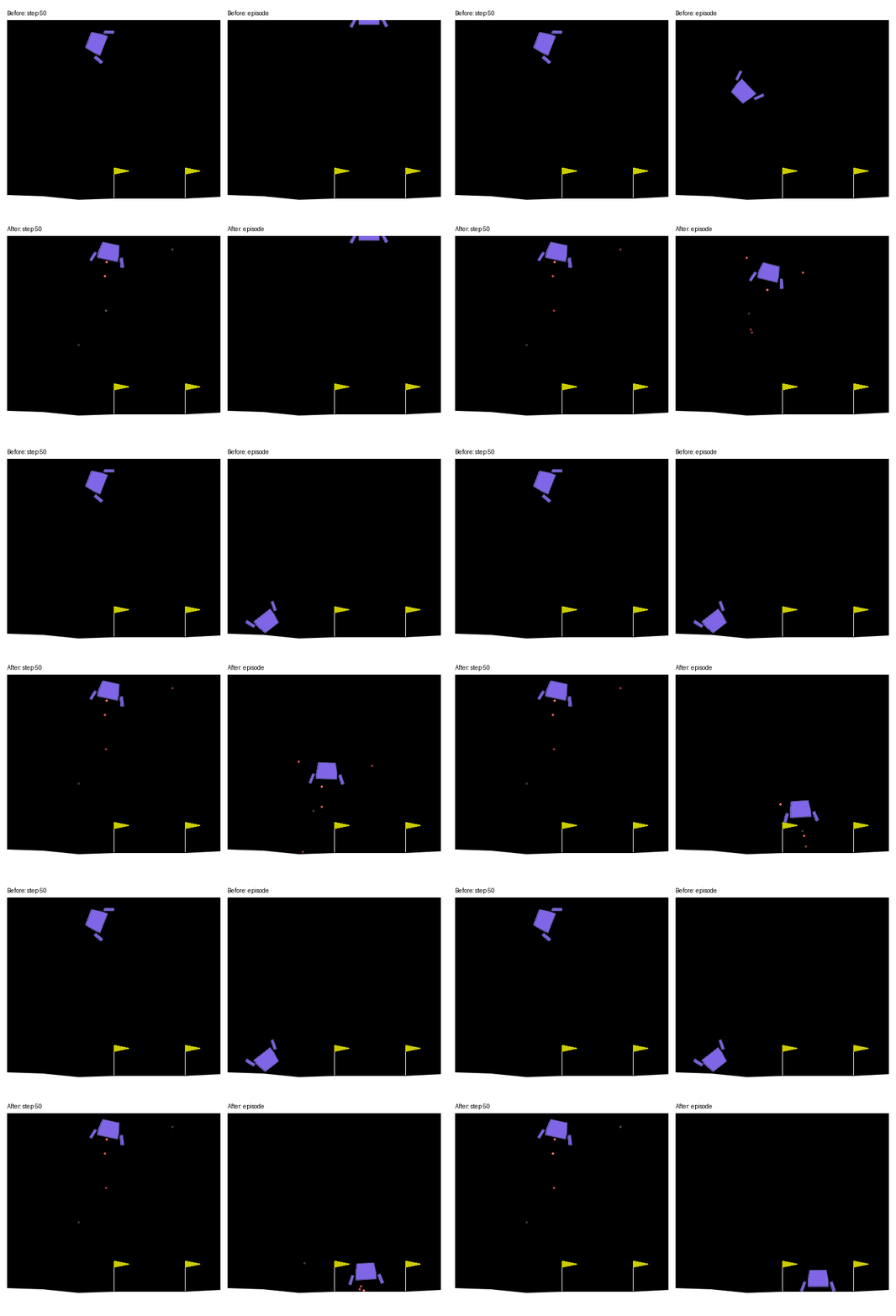
To move from CartPole to LunarLander, we changed the environment, network dimensions and training settings. The PPO update stayed the same.
12.9 Case Study: Learning from Pixels
In LunarLander, the simulator supplied a compact vector of physical
measurements. What if the observation is an image instead? VizDoom provides a
first-person visual environment for reinforcement learning [10]. We use its basic
scenario, in which an agent moves sideways to aim at a stationary target and fires.
The three actions move left, move right and attack. The agent receives a
positive reward for eliminating the target, while time and missed shots carry
costs.
We return to DQN, replacing the multilayer perceptron by a convolutional network. The bridge produces a grayscale screen. Averaging each block gives a observation in . We stack four consecutive frames as channels, so changes between frames are available to the network. Each selected action is repeated for four simulator tics:
  let make seed =
    Doom.S.make ~downsample:4 ~seed "basic"
    |> Frame_stack.S.wrap ~frames:4 in
  let network = N.cnn ~seed:rngs.network_seed ~shape:[|30;40;4|]
      ~convs:[4,2,8; 3,2,16] ~hidden:[64] ~outputs:3 in
The convolution specifications are triples of kernel size, stride and output channels. Thus the first layer uses eight filters with stride two, and the second uses sixteen filters with stride two. After flattening and a hidden layer, the network outputs three action values. It receives no target coordinates or privileged game-state variables.
The replay buffer holds 5,000 transitions. Learning starts after 512 steps; the target network is copied every 1,000 steps. Exploration falls from one to over the first 10,000 steps. We use a smaller learning rate than in the CartPole example:
let total_steps = 2_048  (* Figure: 50_000 *)
let seed = 0
let config = { Dqn.S.default with gamma = 0.95;
  learning_rate = 0.0001; capacity = 5000; batch_size = 32;
  learning_starts = 512; target_every = 1000;
  epsilon_end = 0.1; exploration_steps = 10_000 }
  let raw = make (Random.State.bits rngs.env) in
  let env = { raw with Ndenv.step = (fun action ->
    let st = raw.step action in { st with reward = st.reward *. 0.01 }) } in
  let curve = Dqn.S.train ~config ~steps:!steps ~rngs ~network env in
The default program runs 2,048 steps, enough to exercise sampling, replay and
gradient updates. For Fig. 12.10, set total_steps to 50_000, or pass --steps
50000 to the compiled program. The --frames option records before/after evaluation
frames and saves the final network weights. VizDoom results need not be bitwise
identical across machines.
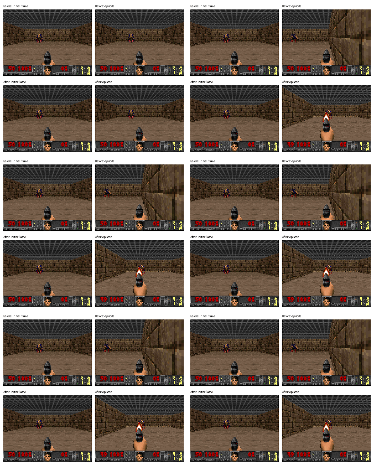
Our first run used . After 50,000 steps, its greedy evaluation return was , compared with before training. It mostly moved rather than making useful attacks. We then changed only the discount factor to , keeping the network, seed, step budget and other settings fixed. The resulting mean evaluation return was on the same 20 evaluation episodes. Reloading the saved weights reproduced that mean, and all 20 episodes ended by eliminating the target rather than reaching the time limit. Some successful episodes still had negative returns because they took many actions or missed shots.
Reducing gives more weight to nearby rewards and costs, changing the objective as well as the learned behaviour. Figure 12.11 compares the first evaluation episode before and after training.
12.10 How owl-rllib Connects to Owl
To follow a neural learning update, start with the environment: reset and step
provide observations and rewards. A replay or rollout buffer stores this experience for
training. The network processes the observations. Policy-gradient methods also use a
distribution to sample actions and compute differentiable probabilities. Each
algorithm constructs its loss and updates the parameters in its own module, so its
update rule can be read in one place. The neural interfaces use Owl ndarrays for
observations and keep the action type explicit; finite MDPs provide transition tables
for planning.
12.10.1 Networks, Differentiation and Explicit Updates
A neural algorithm is a functor over Owl’s graph interface. The ready-made S and D
instances use single- and double-precision arrays respectively. A custom training loop
can use the same choice:
module N = Neural.Make (Owl.Neural.S.Graph)
module AD = N.Algodiff
module Stepper = N.Stepper
Graph constructs and evaluates the network, Algodiff
builds and differentiates the loss, and Optimise.Stepper maintains optimiser state
across updates. The following compiled excerpt shows how a batch loss connects to
that state:
let make_optimiser network =
  Stepper.init (N.adam 0.001) (N.Graph.mkpri network)

let train_batch network observations targets optimiser =
  let predictions, _ = N.Graph.forward network observations in
  let loss = AD.Maths.(mean (sqr (predictions - targets))) in
  N.update network optimiser loss
The optimiser is initialised once for a training run and reused. Reinitialising Adam at every batch would discard its moment estimates. This explicit loop is useful in RL, where collecting a rollout and updating a network alternate, and the target may come from a separate model.
A loss should be expressed using differentiable operations. For example, PPO’s
clipping can be written using min2 and max2 in Maths:
let clipped_loss ~clip ~log_prob ~old_log_prob ~advantages =
  let open AD in
  let ratio = Maths.exp Maths.(log_prob - old_log_prob) in
  let bounded = Maths.(min2 (max2 ratio (F (1. -. clip))) (F (1. +. clip))) in
  Maths.(neg (mean (min2 (ratio * advantages) (bounded * advantages))))
We hold the old log probabilities and advantages fixed while differentiating the loss. Current log probabilities belong to the policy’s differentiation graph. Categorical distributions use log-softmax to compute log probabilities directly. This avoids taking the logarithm of probabilities that may have underflowed to zero.
A DQN target or a language-model reference needs independent parameters:
let target_network online = N.Graph.copy online
A simple OCaml binding to the same network value would share mutable state. An explicit copy expresses the intended separation between online updates and fixed targets.
12.10.2 Randomness and External Environments
Rng.create derives separate streams for environment dynamics, actions, replay
sampling and evaluation, together with a network-initialisation seed. This prevents
an extra evaluation sample from consuming the training action stream. Owl’s
network initialisation still uses Owl’s global random generator, which the network
constructor seeds explicitly.
The Gymnasium and VizDoom bridges run Python in a child process. Numerical observations and rewards cross a line-based protocol using hexadecimal floating-point strings, preserving the transmitted floating-point values exactly. This avoids loading the simulator’s numerical libraries into the OCaml process. The receiver converts these values to the observation array’s precision. The optional frame interface transfers pixel bytes for illustrations without advancing the simulation.
Correctness checks operate at several levels. Fixed action sequences compare environment trajectories with Gymnasium. Analytic and PyTorch reference calculations compare probability distributions, losses and gradients. Small learning tasks check that the algorithms actually update useful parameters. Finally, the chapter examples execute complete learning loops and inspect their results.
Separate five-seed checks give broader performance context: DQN on CartPole reached a mean training return of , compared with in the published CleanRL results. In local LunarLander runs with the same million-step budget and hyperparameters, PPO reached a mean evaluation return of , compared with SB3’s ; the companion notes give the configurations, variation across seeds and evaluation procedures [11].
Planning, learning values, and learning policies use different sources of information, but share a small collection of mathematical operations. Owl supplies these operations; the RL layer determines how experience becomes a target and when the parameters should change.
Bibliography
- [1]
- Sutton RS, Barto AG. Reinforcement Learning: An Introduction. 2nd ed. MIT Press; 2018.
- [2]
- UC Berkeley CS188. Introduction
to Artificial Intelligence: Markov Decision Processes and Reinforcement
Learning.
https://inst.eecs.berkeley.edu/~cs188/textbook/. Accessed 13 November 2026. - [3]
- Mnih V, Kavukcuoglu K, Silver D, et al. Human-level control through deep reinforcement learning. Nature. 2015;518:529–533. doi:10.1038/nature14236.
- [4]
- Williams RJ. Simple statistical gradient-following algorithms for connectionist reinforcement learning. Machine Learning. 1992;8:229–256. doi:10.1007/BF00992696.
- [5]
- Schulman J, Moritz P, Levine S, Jordan MI, Abbeel P. High-dimensional
continuous control using generalized advantage estimation. ICLR; 2016.
https://arxiv.org/abs/1506.02438. - [6]
- Schulman J, Wolski F, Dhariwal P, Radford A, Klimov O. Proximal policy
optimization algorithms. 2017.
https://arxiv.org/abs/1707.06347. - [7]
- Wolfe CR. Reinforcement Learning
for LLMs: The Complete Guide. Deep (Learning) Focus; 24 August 2026.
https://cameronrwolfe.substack.com/p/llm-rl. - [8]
- Shao Z, Wang P, Zhu Q, et al. DeepSeekMath: Pushing the
limits of mathematical reasoning in open language models. 2024.
https://arxiv.org/abs/2402.03300. - [9]
- Farama Foundation. Gymnasium documentation: Lunar Lander.
https://gymnasium.farama.org/v0.29.0/environments/box2d/lunar_lander/. Reference implementation: Gymnasium 0.29.1. - [10]
- Kempka M, Wydmuch M, Runc G, Toczek J, Jaśkowski W. ViZDoom:
A Doom-based AI research platform for visual reinforcement learning.
IEEE Conference on Computational Intelligence and Games; 2016.
https://arxiv.org/abs/1605.02097. - [11]
- Owl RL project. Supplementary experiments: token termination,
baselines and reference implementations. Companion
code,
code/chap17_rl/notes/historical-experiments.md.https://github.com/owlbarn/springer-book-code/tree/main/code/chap17_rl/notes.