CHAPTER 11
Neural Network
Originally conceived as far back as the 1940s, neural networks have received a lot of attention in recent years due to frequently astounding results. In this chapter, we will demonstrate step by step how to build up a practical neural network module with what we have learned so far, especially algorithmic differentiation, optimisation, and regression. After that, we will further present Owl’s neural network module, including its design and usage. After studying the basic feedforward neural network, we will introduce some more advanced types of neural networks, including the Convolutional Neural Network, the Recurrent Neural Network, and the Generative Adversarial Network.
The original idea of a “neural network” comes from attempts by researchers to model how biological neural systems work. The signal processing neurons carry out is modelled as computation, and the complex transmission and triggering of impulses are simplified to activations. In this chapter we start with the simplest neuron, the perceptron, and then go on to introduce how neural networks can be built using regression as previously introduced in Chap. 10. We then proceed to introduce the neural network module from Owl, and three popular types of neural network it supports: convolutional neural network, recurrent neural network, and generative adversarial network. We will give each a quick introduction before concluding this chapter.
11.1 The Perceptron
Before diving into the complex neural network structures, let’s briefly recount the simplest form of neural network: the perceptron. Its definition is actually very similar to that of logistic regression. Recall that logistic regression prediction function can be expressed as:
where is a sigmoid function, . This function maps a finite real number into . A perceptron instead applies a step function to the score :
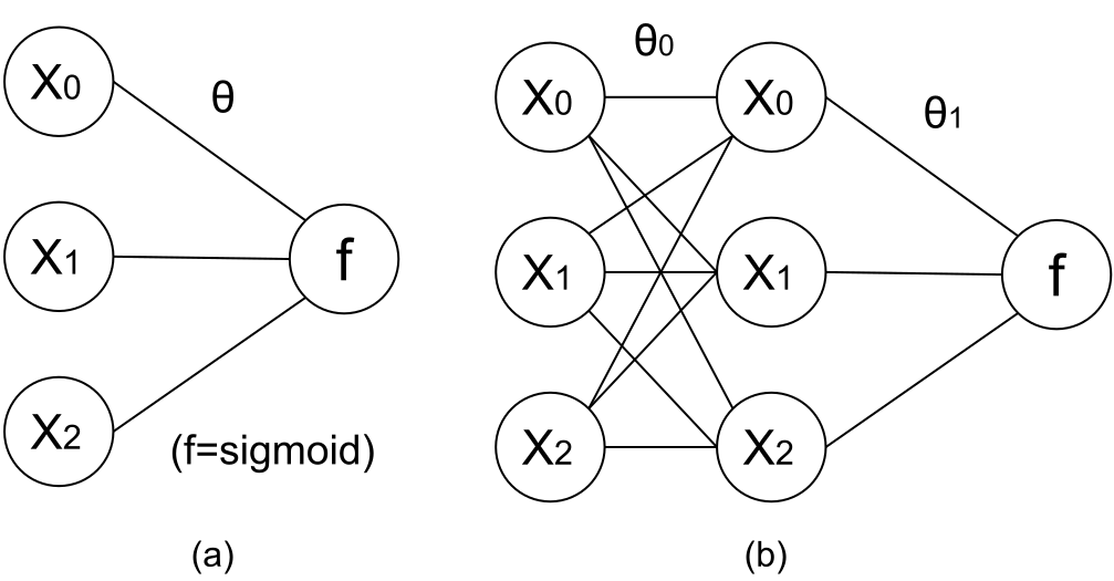
Here denotes the collection of parameters and . The formula uses column vectors; the code stores examples as rows and multiplies on the right. The ten sigmoid outputs are separate scores and need not sum to one. It can be implemented as:
open Algodiff.D
module N = Dense.Ndarray.D

let input_size = 28 * 28
let hidden_size = 25
let classes = 10

let theta0 = Arr (N.uniform ~a:(-0.075) ~b:0.075 [|input_size; hidden_size|])
let theta1 = Arr (N.uniform ~a:(-0.075) ~b:0.075 [|hidden_size; classes|])

let h theta0 theta1 x =
  let t = Arr.dot x theta0 |> Maths.sigmoid in
  Arr.dot t theta1 |> Maths.sigmoid;;
That’s it. We can now classify an input image, flattened into 784 values, into one of the ten classes ... except that we can’t really because the parameters are set to random values. To actually be able to perform the classification accurately, we need to train the model to discover suitable values for and .
11.2.3 Back Propagation
Training a network is essentially the minimisation of the cost function by adjusting the weights of each layer. The core of training is the back propagation which, as introduced in Chap. 8, propagates derivatives from the scalar loss back through the recorded computation graph using the chain rule. Back propagation is especially useful for functions where the number of parameters is far larger than the number of outputs – as is the case with neural networks.
Back propagation [3] is thus central to gradient-based neural network training,
and we can easily build up to it from scratch with the help of AD module. Recall from
Chap. 10 that training is the process of iteratively seeking the parameters
that minimise the cost function. In the case of this neural network, its cost
function is similar to that of logistic regression (Eq. 10.18). Assuming we have
training data pairs, and
outputs, with input
and label matrices
and ,
the mean cost can be expressed as:
until it converges, and the same applies here. Rather than deriving every chain-rule term by hand, we can calculate the derivatives of both parameter matrices using the AD module, and we have shown in Chap. 8 how it can be done in OCaml:
let images,_,labels=Dataset.load_mnist_train_data ();;
let x',y'=Dataset.draw_samples images labels 1;;
let x'=Dense.Ndarray.Generic.cast_s2d x' |> fun x -> N.div_scalar x 255.;;
let y'=Dense.Ndarray.Generic.cast_s2d y';;
let t=tag ();;
let t0=make_reverse theta0 t and t1=make_reverse theta1 t;;
let cost=c t0 t1 (Arr x') (Arr y');;
reverse_prop (F 1.) cost;;
let theta0'=adjval t0 |> unpack_arr;;
let theta1'=adjval t1 |> unpack_arr;;
This first example uses double precision, so the sampled float32 images and labels are converted explicitly. Images are flattened and scaled from – to –; the weights are tagged before reverse propagation. That’s it for one iteration. We get , and can iteratively update the and parameters.
11.2.4 Feedforward Network
The example shows how to obtain gradients, but its structure has several limitations which we will now address.
11.2.5 Layers
The first problem is that the previous example mixes all the primitive computations together. We should add the abstraction of a layer as the building block of a neural network rather than manually encoding so many basic computations. The following code defines the layer and network types as OCaml records. Note that for each layer we add an extra bias parameter alongside the matrix multiplication. This bias vector provides an offset shared across examples. Each fully connected layer with an activation performs the calculation in Eq. 11.2 where is a non-linear activation function.
| (11.2) |
Each layer consists of three components: weight w, bias b, and activation function a.
A network is then just a collection of layers.
open Algodiff.S

type layer = {
  mutable w : t;
  mutable b : t;
  mutable a : t -> t;
}

type network = { layers : layer array };;
Despite the complicated internal structure, we can treat a neural network as a function that takes input data and generates predictions. The question is how to evaluate a network, by decomposing it into a sequence of evaluations of each layer. The output of one layer is given as input to the next layer, propagating forwards until it reaches the network’s output layer. The following two lines show how to evaluate a neural network in a forward pass, which is distinct from forward-mode differentiation.
let run_layer x l = Maths.((x *@ l.w) + l.b) |> l.a
let run_network x nn = Array.fold_left run_layer x nn.layers;;
The run_network function computes the equivalent of the
function in the previous section.
11.2.6 Activation Functions
Let’s step back and check again the similarity between a neural network and our simplified picture of biological neurons. So far we have connected every computation node (or “neuron”) to every node between two layers, but that’s hardly how real neurons work. Rather than activating all connecting neurons during information transformation, different neurons are activated differently in an irregular fashion. Biology aside, think about it mathematically: if we stack fully connected layers without non-linear activations, their matrix multiplications and biases collapse to a single affine transformation.
Therefore, to make adding more layers actually mean something, we frequently
use activation functions to simulate how neurons work in biology, introducing
non-linearity into the network. Non-linearity is a useful property in our models as
most real world data demonstrate non-linear features. In fact, we have already
seen two types of activation function! The first is the Unit Step Function,
which works like a simple on/off gate. Its derivative is zero away from the
threshold and undefined there, so it is unsuitable for ordinary back propagation.
The second is the familiar sigmoid function which maps finite inputs into
. At a
binary output it can model a class probability; a hidden activation need not have
a probabilistic interpretation. There are many other types of non-linear
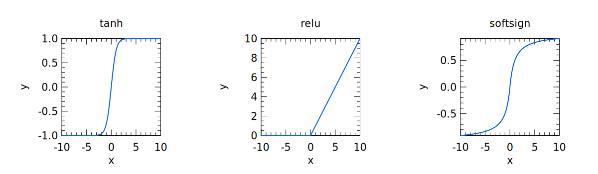
activation functions, shown in Fig. 11.2. The tanh(x) function computes
. Softsign
computes .
The relu(x) computes:
We will keep using these activation functions in later network structures.
11.2.7 Initialisation
In this small example we use only two layers, l0 and l1. l0 uses a
matrix as weights, and tanh as its activation function. l1 is the output layer and
softmax is its activation function.
let l0 = {
  w = Maths.(Mat.uniform 784 40 * F 0.15 - F 0.075);
  b = Mat.zeros 1 40;
  a = Maths.tanh;
}
let l1 = {
  w = Maths.(Mat.uniform 40 10 * F 0.15 - F 0.075);
  b = Mat.zeros 1 10;
  a = Maths.softmax ~axis:1;
}
let nn = {layers = [|l0; l1|]};;
let handwritten_nn=nn;;
In Chap. 10 we saw that finding a good initial starting point for parameter values can be beneficial to the performance of gradient descent. Uniform or Gaussian random values can work well, but their scale matters.
If the initial weights are too large, pre-activation values can grow across layers and drive sigmoid units close to either 0 or 1, where their derivatives are small. Very small weights can also make back-propagated gradients shrink across layers. Vanishing gradients refer to small derivatives, not simply small network outputs; for example, sigmoid at zero is 0.5. In either case training can become inefficient.
There have been many attempts to address these difficulties [4] [16] [5]. ReLU
avoids saturation on its positive side, though it does not solve every gradient
problem. As to initialisation itself, there are multiple heuristics. For a dense layer
with
inputs, Owl’s Init.Standard samples uniformly from
. This is
not the Xavier/Glorot rule. Init.LecunNormal uses a zero-mean Gaussian with standard
deviation .
Xavier/Glorot initialisation [6] takes both the input size
and output
size into
account. Init.GlorotNormal uses a zero-mean Gaussian with standard deviation
. Init.GlorotUniform
samples uniformly from ,
where ;
Init.Tanh is an alias for this rule. These are useful choices for tanh
layers. Our small hand-written example above uses the fixed interval
instead. Owl also provides Init.Uniform and Init.Gaussian with explicit
distribution parameters, and Init.Custom, which accepts a function from the weight
shape to an initial parameter array.
11.2.8 Training
The loss function is constructed by executing a forward pass through the network as the code below shows. This version uses softmax outputs with categorical cross-entropy: the outputs sum to one, and only the true class contributes to each one-hot loss. Unlike the earlier independent-sigmoid example, no complementary label term is needed.
let loss_fun nn x y =
  let t = tag () in
  Array.iter (fun l ->
    l.w <- make_reverse (primal' l.w) t;
    l.b <- make_reverse (primal' l.b) t;
  ) nn.layers;
  Maths.(cross_entropy y (run_network x nn) /
    (F (Mat.row_num y |> float_of_int)));;
The backprop function uses the same procedure as the previous example. Reverse
propagation computes the derivatives, which are retrieved using adjval, and the
parameter w and b of each layer are updated accordingly. It then uses the
gradient descent method; for simplicity, the learning rate eta is fixed to a
constant.
let backprop nn eta x y =
  let loss = loss_fun nn x y in
  reverse_prop (F 1.) loss;
  Array.iter (fun l ->
    l.w <- Maths.((primal l.w) -
      (eta * (adjval l.w))) |> primal;
    l.b <- Maths.((primal l.b) -
      (eta * (adjval l.b))) |> primal;
  ) nn.layers;
  loss |> unpack_flt;;
11.2.9 Test
Now we have all these parts in place, we can finally see how well our trained
model works. The test function performs model inference and compares the
predictions with labelled data. By doing so, we can evaluate the accuracy of a neural
network.
let test nn x y =
  Dense.Matrix.S.iter2_rows (fun u v ->
    let p = run_network (Arr u) nn |> unpack_arr in
    Dense.Matrix.Generic.print p;
    let _, prediction = Dense.Matrix.Generic.max_i p in
    let _, label = Dense.Matrix.Generic.max_i v in
    Printf.printf "prediction: %i label: %i correct: %b\n"
      prediction.(1) label.(1) (prediction.(1) = label.(1))
  ) (unpack_arr x) (unpack_arr y);;
To put all these parts together, the following code starts the training for
999 iterations. We use the Dataset module in Owl to load training and
test data, and draw a certain number of samples randomly from the loaded
data.
let main () =
  let x, _, y = Dataset.load_mnist_train_data () in
  let x=Dense.Matrix.S.div_scalar x 255. in
  for i = 1 to 999 do
    let x', y' = Dataset.draw_samples x y 100 in
    backprop nn (F 0.01) (Arr x') (Arr y')
    |> Owl_log.info "#%03i : loss = %g" i
  done;
  let x, _, y = Dataset.load_mnist_test_data () in
  let x=Dense.Matrix.S.div_scalar x 255. in
  let x, y = Dataset.draw_samples x y 10 in
  test nn (Arr x) (Arr y);;
main ();;
The hand-written network uses flat, normalised images and float32 arithmetic. The third dataset result is the one-hot label matrix used for testing, matching the network’s ten outputs.
When the training starts, our code keeps printing the value of loss function after each update, reporting the batch loss computed before that update. The excerpt below comes from the actual 999-iteration run. Loss is evaluated on randomly drawn batches, so individual values can fluctuate; running the complete example produces the full log.
#001 : loss = 2.3172
#002 : loss = 2.29518
#003 : loss = 2.3094
#004 : loss = 2.28527
#005 : loss = 2.29251
#006 : loss = 2.29086
#007 : loss = 2.28063
#008 : loss = 2.28878
...
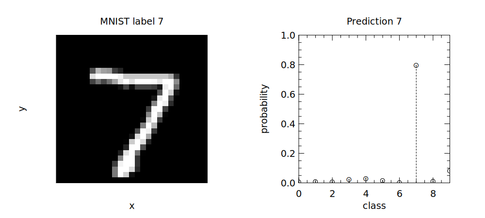
After training is finished, we test the accuracy of this network. Here is an example using the first test image. The left panel shows the input and its true label; the right panel shows the network’s output probabilities for all ten digits and its predicted label.
11.3 Neural Network Module
The simple implementation we built in the previous section looks promising, but
a neural network library cannot really leave it for the users to define so
much for themselves. Owl provides the Neural Network module Neural, the
use of which is actually very similar to the naive framework we just built,
but with an improved API and more complete support for various types
of neuron. In this section we introduce both how to use it and how it is
built.
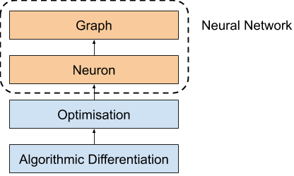
Fig. 11.4 shows the basic architecture of the neural network module in the Owl
library. The neural network module mainly consists of two submodules, Neuron and
Graph, built on the optimisation module, which in turn is built on the Algorithmic
Differentiation module. As we have seen in the previous section, for neural networks
we need only describe the logic of the forward pass while derivatives of the supported
operations are handled by Algodiff figuring it out automatically for us, reducing the
potential for errors.
11.3.1 Neurons
Owl uses the term neuron for modules that encapsulate layer operations, such as
a whole fully connected layer, rather than only a single scalar unit. In this section, we
will explain the internal structure of a neuron module. We have already seen how the
input and hidden layers can be connected; such computation can be abstracted into
the FullyConnected neuron module, the type definition of which is shown
below.
open Neural.S;;
open Neural.S.Graph;;
open Neural.S.Graph.Neuron;;
open Neural.S.Algodiff;;
module FullyConnected=Neural.S.Graph.Neuron.FullyConnected;;
open FullyConnected;;

type neuron_typ =
  Owl_neural_generic.Make_Embedded(Owl_algodiff_primal_ops.S).Neuron.FullyConnected.neuron_typ = {
  mutable w : Owl_neural.S.Graph.Neuron.Optimise.Algodiff.t;
  mutable b : Owl_neural.S.Graph.Neuron.Optimise.Algodiff.t;
  mutable init_typ : Owl_neural.S.Graph.Neuron.Init.typ;
  mutable in_shape : int array;
  mutable out_shape : int array;
}
This module contains the two parameters we have seen: w and b, both of type t,
the Algodiff value type used here for arrays. To use this neuron, we need to specify
its input and output shape. They are actually the length of input vector and the
length of the hidden layer itself. The last part in the definition of this neuron
init_typ describes the initialisation used. After the type definition, this
module contains several standard functions that are shared by all the neuron
modules.
let create ?inputs o init_typ =
  let in_shape =
    match inputs with
    | Some i -> [| i |]
    | None   -> [| 0 |]
  in
  { w = Mat.empty 0 o; b = Mat.empty 1 o;
    init_typ; in_shape; out_shape = [| o |] };;
create function. Here
we specify the output size o and the initialisation method; the input size is optional
at creation time.
let connect out_shape l =
  assert (Array.length out_shape > 0);
  l.in_shape <- Array.copy out_shape;;
connect function. We will see why we need the connect function later. Next we
initialise the parameters:
let init l =
  let m = Array.fold_left (fun a b -> a * b) 1 l.in_shape in
  let n = l.out_shape.(0) in
  l.w <- Init.run l.init_typ [| m; n |] l.w;
  l.b <- Mat.zeros 1 n;;
m is a flattened input size in case input ndarray is of multiple dimensions.
The w parameter is initialised with predefined initialisation function, and we can just
make b all zero, which means no bias at the beginning. Then we build the forward
propagation procedure, in the run function:
let run x l =
  let m = Mat.row_num l.w in
  let n = Arr.numel x / m in
  let x = Maths.reshape x [| n; m |] in
  let y = Maths.((x *@ l.w) + l.b) in
  y;;
Finally, we divide back propagation into several parts: tagging the parameters, obtaining derivatives, and updating parameters. They are also included in the neuron module:
let mktag t l =
  l.w <- make_reverse l.w t;
  l.b <- make_reverse l.b t

let mkpri l = [| primal l.w; primal l.b |]

let mkadj l = [| adjval l.w; adjval l.b |]

let update l u =
  l.w <- u.(0) |> primal';
  l.b <- u.(1) |> primal';;
That’s about all for the structure of the FullyConnected neuron, and the other
neurons share the same or very similar structure. Similar to other modules such as
Ndarray and Algodiff, the Neural module provides S and D for single and double
precision. The neuron modules used here are under Neural.S.Graph.Neuron (or the
corresponding double-precision path).
Neural Graph
The neuron is the core of the neural network module but we do not work directly
with neurons but with neural networks, where individual neurons are instantiated
into nodes and connected into a graph using the Graph module. A node in a neural
network is composed of multiple parts:
type node =
  Owl_neural_generic.Make_Embedded(Owl_algodiff_primal_ops.S).node = {
  mutable name : string;
  mutable prev : Owl.Neural.S.Graph.node array;
  mutable next : Owl.Neural.S.Graph.node array;
  mutable neuron : Owl.Neural.S.Graph.Neuron.neuron;
  mutable output : Owl.Neural.S.Graph.Neuron.Optimise.Algodiff.t option;
  mutable network : Owl.Neural.S.Graph.network;
  mutable train : bool;
}
Besides the neuron itself, a node also contains information such as its
parents, children, output, the network it belongs to, a flag if this node is only
for training, etc. In the Graph module, most of the time we need to deal
with functions that build a node and connect it to existing network. For
example:
let fully_connected ?name ?(init_typ = Init.Standard) ?act_typ
  outputs input_node =
  let neuron = FullyConnected
    (FullyConnected.create outputs init_typ) in
  let nn = get_network input_node in
  let n = make_node ?name [||] [||] neuron None nn in
  add_node ?act_typ nn [| input_node |] n;;
This function instantiates the FullyConnected neuron using its create function,
and wraps it into a node n. The current network nn is built from its input node
input_node. Then we add n as a child node to nn and connect it to its
parents using the add_node function. This step uses the connect function of
the neuron, and also updates the child’s input and output shape during
connection.
Finally, after understanding the Graph module, we can now re-define the network
in previous example with the neural network module:
open Neural.S
open Neural.S.Graph
open Neural.S.Algodiff

let make_network () =
  input [|28; 28; 1|]
  |> fully_connected 40 ~act_typ:Activation.Tanh
  |> linear 10 ~act_typ:Activation.(Softmax 1)
  |> get_network;;
The code above shows how convenient this module makes building neural
networks. We can see how the input, the hidden layer, and the output from the
previous example are concisely expressed. The linear layer in the code is similar to
fully_connected, except that each example must already be a vector; the full input
still includes a batch dimension. The parameter act_typ specifies the activation
function applied on the output of this node.
This network definition starts with an input layer and ends with get_network,
which returns the constructed network. Here the input shape is fixed as
[|28;28;1|], excluding the batch dimension. The downstream shapes are
inferred as nodes are connected, saving effort and reducing shape errors.
Parameter values are initialised separately by Graph.init or when training
begins.
11.3.2 Training Parameters
After a network is built, the last thing to do is to train the model by learning the
weights. Again, we want to encapsulate all the manual back-propagation and
parameter update into one simple function, primarily implemented in the
minimise_network function in the Optimise module. This module provides the
Params sub-module which maintains a set of training hyper-parameters. To avoid
diving too deeply into the sea of implementation details, we focus on one update, the
-th
iteration, and see how these hyper-parameters work. Let’s start with the first step in
this iteration: training data batching.
The following internal steps use a small MNIST slice to make their batch and network context explicit.
let network=make_network ();;
Graph.init network;;
let raw_x,_,raw_y=Dataset.load_mnist_train_data ();;
let small_x=Dense.Matrix.S.get_slice [[0;99];[]] raw_x |> fun x -> Dense.Matrix.S.div_scalar x 255.;;
let small_y=Dense.Matrix.S.get_slice [[0;99];[]] raw_y;;
let x=Arr (Dense.Ndarray.S.reshape small_x [|100;28;28;1|]) and y=Arr small_y;;
let params=Params.config ~batch:(Batch.Mini 10) ~regularisation:(Regularisation.L2norm 0.001) 1.;;
let batch_fun=Optimise.Batch.run params.batch;;
let i=0;;
let forward=Graph.forward network;;
let loss_fun=Optimise.Loss.run params.loss;;
let regl_fun=Optimise.Regularisation.run params.regularisation;;
module Regularisation=Optimise.Regularisation;;

let xt, yt = batch_fun x y i;;
We use Batch module to specify how the training data are batched. In the
definition of cost functions, we often assume that we must include all the data when
updating parameters, described using the type constructor Batch.Full.
However, for large scale training tasks, there might be millions of points
of training data, which can not only cause memory issues but often also
requires waiting for all the data to be processed to get a single parameter
update.
The most commonly used batching method is mini-batch, Batch.Mini, which uses
only a small part of the training data [7]. Mini-batch updates are not equivalent to a
full-batch update, because the parameters change between batches. A randomly
sampled batch can estimate the full-data gradient at the current parameters, allowing
more frequent updates at lower cost.
If we continue the process to its ultimate end where only one data sample is used
each time, we are using the stochastic batch method, Batch.Stochastic.
Single-sample updates can be useful, but make less use of vectorised computation
than larger batches.
A final batching approach is Batch.Sample which is the same as mini-batch
except that each batch is randomly sampled, whereas Batch.Mini takes consecutive
chunks and does not itself shuffle the data. This is particularly useful if the training
data are presented in some kind of order. For example, imagine that the training data
for the MNIST task are ordered according to the digit value – you might end up
with a model that only works for the lower digits like 0, 1, and 2 at the
beginning.
let yt', ws = forward xt;;
Next, the forward function executes the computation layer by layer,
accumulating the result in yt’, which is not simply an ndarray but an Algodiff data
type that records the dependencies needed for reverse propagation. The ws is a
nested array of parameters in the neural network.
let loss = loss_fun yt yt'
let loss = Maths.(loss / _f (Mat.row_num yt |> float_of_int));;
To compare how different the inference result y’ is from the true label y, we
need a loss function. Previously we have used the cross_entropy, but the
Loss module provides other popular loss functions [8]. For residual elements
, their
current definitions are:
Loss.L1norm:Loss.L2norm:Loss.Quadratic:Loss.Hinge: , with labels or .
In Chap. 10 we talked about regularisation and its benefits, introducing different types of regularisation methods.
The Regularisation sub-module is provided in the optimisation module, and
we can use L1norm, L2norm, or Elastic_net regularisation methods [9] in
training. We can also choose not to apply regularisation method by using the
None parameter. As in Chap. 10, Owl’s L2 penalty is the unsquared norm,
including the L2 part of Elastic_net. The code below applies the penalty to
each parameter array, including biases, and adds it to the batch-averaged
loss.
let reg =
  match params.regularisation <> Regularisation.None with
  | true  -> Owl_utils.aarr_fold
    (fun a w -> Maths.(a + regl_fun w)) (F 0.) ws
  | false -> _f 0.
let loss = Maths.(loss + reg);;
The Graph module provides a train function that is a wrapper of this
optimisation function. As a result, we can train the network by simply calling the
train function.
let train () =
  let x, _, y = Dataset.load_mnist_train_data_arr () in
  let x=Dense.Ndarray.S.div_scalar x 255. in
  let network = make_network () in
  let params = Params.config
    ~batch:(Batch.Mini 100)
    ~learning_rate:(Learning_Rate.Adagrad 0.005) 0.1
  in
  Graph.train ~params network x y |> ignore;
  network;;
let trained_network=train ();;
The train function uses the Learning_Rate sub-module. Until now we have been
using constant learning rates, Learning_Rate.Const, but this has problems: we want
the gradient descent to be fast using large steps when training starts, decreasing
to use small steps as it closes in on the minimum point so we can avoid
overshooting. To achieve this we have the Decay and Exp_decay learning rate
methods which both reduce the base learning rate according to the iteration
number [10].
The first reduces the learning rate by a factor of , where is the iteration number and is the reduction rate; the second reduces the learning rate by a factor of .
The Learning_Rate.Adagrad [11] method used here adapts the step
size separately for each parameter using a running sum of its past squared
gradients. Parameters with larger accumulated squared gradients receive smaller
effective learning rates; this can be useful for sparse features. RMSprop [12] is a
separate method that replaces this sum with an exponentially decaying average.
Adam [13] maintains averages of both gradients and squared gradients, with bias
correction.
The last thing to notice in the training parameters is the last number, 0.1,
denoting the training epochs or how many times to repeat on the whole
dataset. Here 0.1 sets a total budget of 60 updates with batches of 100,
approximately one tenth of an epoch; it is not the fraction of data used in each
update.
After training is finished, finally we can evaluate the trained network
on the test set by comparing predicted and true labels. The code below
shows how to do that. It is built around the Graph.model function that
generates a functional model to perform inference, given a trained network and
inputs.
let test network =
  let imgs, _, labels = Dataset.load_mnist_test_data () in
  let imgs=Dense.Matrix.S.div_scalar imgs 255. in
  let m = Dense.Matrix.S.row_num imgs in
  let imgs = Dense.Ndarray.S.reshape imgs [|m;28;28;1|] in

  let mat2num x = Dense.Matrix.S.of_array (
      x |> Dense.Matrix.Generic.max_rows
        |> Array.map (fun (_,_,num) -> float_of_int num)
    ) 1 m
  in

  let pred = mat2num (Graph.model network imgs) in
  let fact = mat2num labels in
  let accu = Dense.Matrix.S.(elt_equal pred fact |> sum') in
  Owl_log.info "Accuracy on test set: %f"
    (accu /. (float_of_int m));
  accu /. float_of_int m;;
let graph_accuracy=test trained_network;;
The recorded reference run obtains 83.8% accuracy on all 10,000 test images after the configured 0.1 epoch. This result depends on the initialisation, data order and training settings. More training may improve it, but does not guarantee a particular accuracy.
The Graph module also provides utility functions such as save, load, print, and
to_string to help manipulate the neural network.
11.4 Convolutional Neural Network
So far we have seen how an example of fully connected feedforward neural network evolves step by step. However, there are many other kinds of neural network. In this section we will see how to build a convolutional neural network (CNN) for the same task.
As its name suggests, this neural network uses convolution-like operations related to those in Chap. 7. For one image channel, a 2D filter moves across the image, multiplying the overlapping entries element-wise and summing the products. CNN libraries, including Owl, conventionally call this convolution even though the kernel is not flipped: mathematically it is cross-correlation. With multiple channels, the products are also summed across input channels, and multiple filters produce output channels. Shared local filters are useful for extracting image features.
To build a CNN we need more types of neurons, the most common of which are implemented by the neural network module, including convolution (both 2D and 3D), pooling [14], batch normalisation [15]. These support many commonly used convolutional architectures.
As the MNIST handwritten recognition task is also a computer vision task, let’s try it using a CNN. The code below creates a small convolutional neural network with input scaling, convolution, pooling, dropout and two dense layers.
let make_network input_shape =
  input input_shape
  |> lambda (fun x -> Maths.(x / F 256.))
  |> conv2d [|5;5;1;32|] [|1;1|] ~act_typ:Activation.Relu
  |> max_pool2d [|2;2|] [|2;2|]
  |> dropout 0.1
  |> fully_connected 1024 ~act_typ:Activation.Relu
  |> linear 10 ~act_typ:Activation.(Softmax 1)
  |> get_network;;
The same Graph training interface can be used, but this example only constructs the CNN and checks its forward computation; it does not train or measure its accuracy. Its scaling layer divides raw pixel values by 256, so inputs should not also be divided by 255 as in the preceding example.
As the CNN is such an important driving force in the computer vision field, Part III of this book includes three case studies using it: image recognition, instance segmentation, and neural style transfer. We will see CNN at play with more details in these application cases.
11.5 Recurrent Neural Network
In all the previous examples there is one obvious, perhaps trivial pattern that can be observed – given one input, the trained network generates an output – but not every real world task works like that. Often the input data is a sequence and the output is updated based not on the current input alone but also on earlier inputs from the sequence. For example, if we need to generate English based on French, or label each frame in a video, focusing on only the current word or frame is not enough.
That’s where the Recurrent Neural Network (RNN) [3] comes in, processing sequences and producing either a sequence of outputs or a single output for the whole sequence. The basic structure of an RNN is quite simple: a neural network that passes a hidden state from one time step to the next, enabling information from previous data in the sequence to be retained.
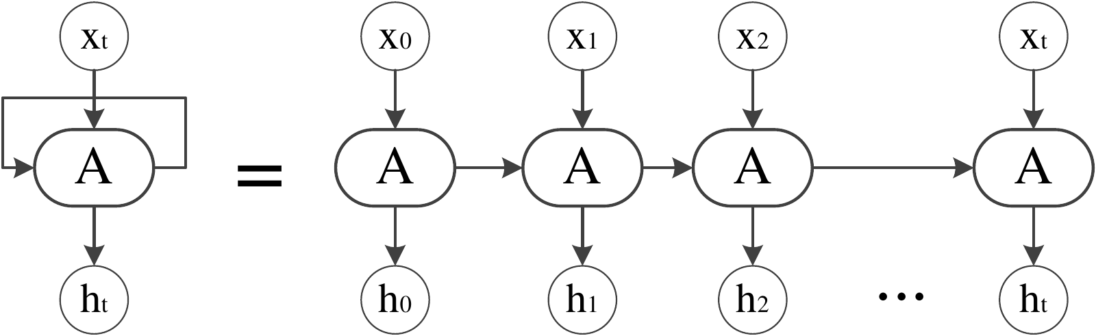
As shown in Fig. 11.5, an RNN can be unrolled into a chain of repeated computations with shared parameters. Here the ’s are sequential inputs, and the ’s are the hidden states, which can be used to produce the outputs of the RNN. The functionality of a RNN therefore mainly relies on the processing logic in .
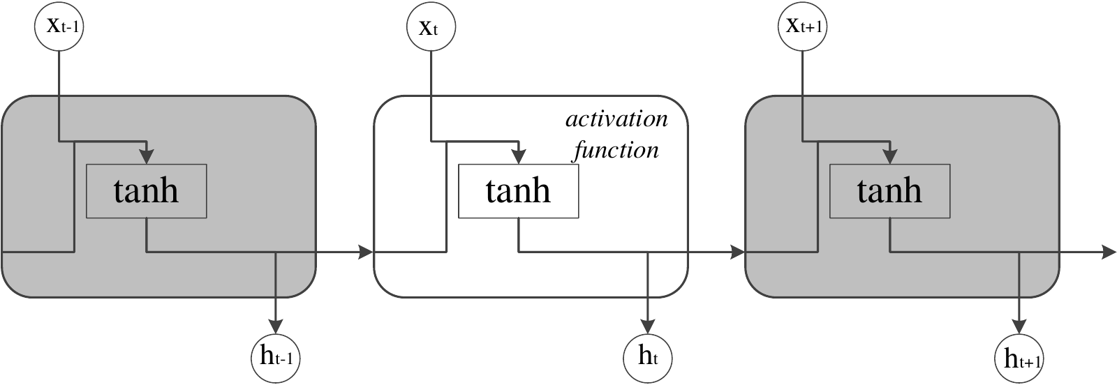
In a vanilla recurrent neural network, the function can be quite simple:
| (11.3) |
This is exactly what we have seen in the feedforward networks. Here
,
and
are
the shared parameters to be trained. Equivalently, the two matrix products can be
written as one matrix multiplying the concatenation of the hidden state and current
input. This process is shown in Fig. 11.6. The activation function in this
calculation is usually the tanh function, so as to keep values within range of
.
However, vanilla RNNs can struggle to learn long-range dependencies: gradients propagated across many time steps may vanish or explode. Gated architectures such as Long Short-Term Memory (LSTM) help address this difficulty.
Proposed by Hochreiter and Schmidhuber in 1997 [16] and widely used and refined by many subsequently, LSTM adds a cell state alongside the hidden state. The commonly used form below also includes the later forget gate [17]. Its basic idea is simple. We still pass in the output from previous loop, but instead of taking it as-is, three choices are made: what to forget, what to remember, and what to output. In this way, useful information from old data can be kept longer, increasing the RNN’s memory.
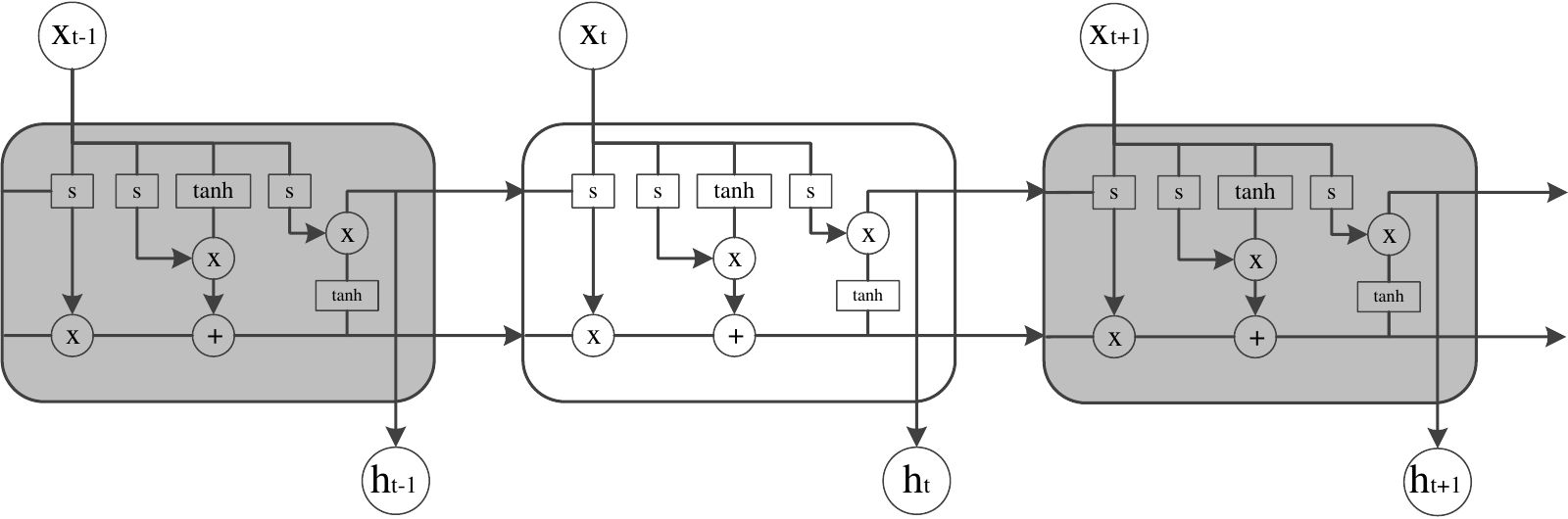
Let’s see how it achieves this effect. The processing unit of LSTM is shown in Fig. 11.7. It consists of three parts that correspond to the three choices listed above. Unlike standard RNN, each unit also takes in and produces a state that flows along the whole loop process. This state is modified twice within the unit.
The first choice is made by the forget gate layer. This combines the hidden state
and the
input ,
and outputs sigmoid gate values to control how much of the existing
information should be kept. These values lie between 0 and 1 and
are computed using the sigmoid activation function, denoted by
.
The second choice is to decide what to remember of the existing data, implemented by
two branches. The first uses the sigmoid function to denote which part of the combined
input
should be updated, and the second uses the tanh function to decide how much value
to update for the vector. The brackets denote concatenation, not addition. Both
branches follow Eq. 11.3, but with different weights, biases and activation
functions.
By multiplying these two branch outputs element-wise, we know how much new information we should add to the information flow . The flow is therefore first multiplied with the output from the forget gate to remove unnecessary information, before adding the output from the second step to gain necessary knowledge.
The final choice is to decide what to output, by once more
running a sigmoid function to decide which part of information flow
to
keep. This is applied as a filter to a tanh-scaled information flow to finally obtain the
output .
LSTM is widely used in time-series related applications such as speech recognition, time-series prediction, human action recognition, robot control, etc. Using the neural network module, we can build an LSTM network that maps a window of token indices to a distribution over the next token. Text generation would additionally require a training corpus, a training loop and repeated sampling. The code below builds the network structure only.
open Neural.S
open Neural.S.Graph

let make_network wndsz vocabsz =
  input [|wndsz|]
  |> embedding vocabsz 40
  |> lstm 128
  |> linear 512 ~act_typ:Activation.Relu
  |> linear vocabsz ~act_typ:Activation.(Softmax 1)
  |> get_network;;
That’s it. The network is even simpler than that of the CNN. Here wndsz is the
input window length and vocabsz is the vocabulary size; the embedding size is 40
and the LSTM hidden size is 128. This Owl LSTM returns the final hidden state,
giving one output distribution per window. The recurrent dependency limits
parallelism across time steps, and training through long sequences can be
costly.
The LSTM has been refined in subsequent work, and there are many variants of it. For example, the Gated Recurrent Unit (GRU) proposed in 2014 [18].
Compared to LSTM, the GRU uses two gates: a “reset gate” that decides how
much information to forget from the past, and an “update gate” behaving like a
combination of LSTM’s forget and input gates. It uses a single hidden state rather
than a separate cell state. At the same hidden size, it usually has fewer parameters
and can be faster, but predictive performance and training time depend on the task
and implementation. In the LSTM code above, we can just replace the lstm node
with gru.
11.6 Generative Adversarial Network
We need to discuss one more type of neural network which isn’t actually a particular type with new neurons like a CNN or RNN, but more of a (huge) family of networks exhibiting a particular pattern: the Generative Adversarial Network (GAN) [19]. The typical target for training a GAN is to automatically learn patterns in the input data so that the model can be used to generate “fake data” that look like they could have been drawn from the original data.
A GAN consists of two competing parts, generator and discriminator, that are constantly at war with each other. During training, the generator tries its best to synthesise data based on existing parameters, and the discriminator tries its best to separate the generated data from the true data. At the ideal equilibrium, the generated and real distributions match and an optimal discriminator outputs 0.5. In practice, training may not reach this equilibrium; fooling the current discriminator does not by itself establish visual realism or diversity.
Let’s look at an example. Previously we have used the MNIST dataset extensively in image recognition task, but now let’s try something different with it. Say we want to build a neural network that can produce a digit picture that looks like it’s taken from the MNIST dataset. It doesn’t matter which digit – the point is simply that it should be realistic and newly generated, rather than a deliberate copy of a training image. The GAN objective alone does not rule out memorisation. To generate such an image does not require a highly complex network structure. For example, we can use something like below:
open Neural.S
open Neural.S.Graph
open Neural.S.Algodiff

let make_generator input_shape =
  let out_size = Owl_utils_array.fold_left ( * ) 1
    input_shape in
  input input_shape
  |> fully_connected 256 ~act_typ:(Activation.LeakyRelu 0.2)
  |> normalisation ~decay:0.8
  |> linear 512 ~act_typ:(Activation.LeakyRelu 0.2)
  |> normalisation ~decay:0.8
  |> linear 1024 ~act_typ:(Activation.LeakyRelu 0.2)
  |> normalisation ~decay:0.8
  |> linear out_size ~act_typ:Activation.Tanh
  |> reshape input_shape
  |> get_network;;
We connect multiple linear layers, activation layers, and normalisation
layers, and don’t even need to use any convolution layers. By now you should
be familiar with this kind of network structure: this example accepts
random noise with shape [|batch;28;28;1|] and outputs greyscale
image-shaped arrays of the same shape. The final tanh maps values to
; real
MNIST images would need matching scaling during adversarial training.
As well as this generator, the other half of the GAN is the discriminator. The structure is also quite simple:
let make_discriminator input_shape =
  input input_shape
  |> fully_connected 512 ~act_typ:(Activation.LeakyRelu 0.2)
  |> linear 256 ~act_typ:(Activation.LeakyRelu 0.2)
  |> linear 1 ~act_typ:Activation.Sigmoid
  |> get_network;;
The discriminator takes in an image as input and outputs only a single value through the sigmoid activation function – its estimated probability that the input comes from the real data rather than the generator. Values near 1 indicate a prediction of real data, and values near 0 indicate generated data; these are predictions, not guarantees.
The question is: how to train these two parts so that they mutually reinforce each
other? We do so by carefully crafting the loss functions. The point of this step is to
make the discriminator distinguish the output from generators from the true images
as effectively as possible. For simplicity, consider one real MNIST image
and one generated image at each step. First, to train the discriminator we
consider the ground truth: we know that the data taken from MNIST must
be true, so it is labelled 1, while we know that anything that comes from
generator, no matter how good it is, must be a fake and so is labelled 0. By
adding these two parts together, we can get a loss value for training the
discriminator.
To train the generator, we use generated samples and reverse our target label. We
combine the generator network and discriminator network together, give it a
random noise image as input, and use 1 as the target for the discriminator
output, even though we know that at the beginning the output from generator
would be obviously not an MNIST image. The loss value is obtained by
comparing the output of this combined network and the target label 1. During
this generator update, we hold the discriminator parameters fixed but still
differentiate through it to the generator. The point of this step is to make
generator produce images that can fool the discriminator as convincingly as
possible.
That’s all. In some ways it is like a small scale Darwinian simulation: the two models improve in response to each other. This is the intended training dynamic, rather than a guarantee of convergence. The code shown here defines the two networks and checks forward outputs; it does not implement this alternating training procedure.
This approach has been successfully applied in many applications, such as Pix2Pix [20], face ageing [21], increasing photo resolution [22], etc. For Pix2Pix, you give it a pencil-drawn picture of a bag and it can render it into a real-looking bag. Or think about the popular application that creates a new anime character [23]. In these applications, the generators are all required to generate plausible images, whether translating an existing image or synthesising a new one. A more thorough introduction to developments in GANs up to 2019 can be seen in Pan et al [24].
11.7 Summary
This chapter gave a detailed introduction to the theory behind neural networks, alongside the implementation of a simple neural network module. Starting with the a basic early form of neural network, the perceptron, we manually built a feedforward network to perform multi-class handwritten digit recognition task by extending logistic regression. Next, we introduced Owl’s Neural Network module, including how its core works and how it is built step by step. We used this module to solve the same example, including training and testing, and explained how to configure initialisation and training parameters. We then introduced two important types of neural network: the convolutional neural network and the recurrent neural network in two of its variants, LSTM and GRU. We finished with a brief introduction to the basic idea behind Generative Adversarial Networks, another type of neural network with many research and application examples.
Bibliography
- [1]
- Rosenblatt F. The perceptron, a perceiving and recognizing automaton Project Para. Cornell Aeronautical Laboratory; 1957.
- [2]
- LeCun Y, Bottou L, Bengio Y, Haffner P. Gradient-based learning applied to document recognition. Proceedings of the IEEE. 1998 Nov; 86(11):2278-324.
- [3]
- Rumelhart DE, Hinton GE, Williams RJ. Learning representations by back-propagating errors. nature. 1986 Oct;323(6088):533-6.
- [4]
- Schmidhuber J. Learning complex, extended sequences using the principle of history compression. Neural Computation. 1992 Mar;4(2):234-42.
- [5]
- He K, Zhang X, Ren S, Sun J. Deep residual learning for image recognition. Proceedings of the IEEE conference on computer vision and pattern recognition 2016 (pp. 770-778).
- [6]
- Glorot X, Bengio Y. Understanding the difficulty of training deep feedforward neural networks. Proceedings of the Thirteenth International Conference on Artificial Intelligence and Statistics. PMLR. 2010;9:249–256.
- [7]
- Li M, Zhang T, Chen Y, Smola AJ. Efficient mini-batch training for stochastic optimization. Proceedings of the 20th ACM SIGKDD international conference on Knowledge discovery and data mining 2014 Aug 24 (pp. 661-670).
- [8]
- Rosasco L, De Vito E, Caponnetto A, Piana M, Verri A. Are loss functions all the same?. Neural computation. 2004 May 1;16(5):1063-76.
- [9]
- Zou H, Hastie T. Regularization and variable selection via the elastic net. Journal of the royal statistical society: series B (statistical methodology). 2005 Apr; 67(2):301-20.
- [10]
- You K, Long M, Wang J, Jordan MI. How does learning rate decay help modern neural networks?. arXiv preprint arXiv:1908.01878. 2019 Aug 5.
- [11]
- Duchi J, Hazan E, Singer Y. Adaptive subgradient methods for online learning and stochastic optimization. Journal of Machine Learning Research. 2011;12(61):2121–2159.
- [12]
- Tieleman, T. and Hinton, G. Lecture 6.5 - RMSProp, COURSERA: Neural Networks for Machine Learning. Technical report. 2012.
- [13]
- Kingma DP, Ba J. Adam: A method for stochastic optimization. arXiv preprint arXiv:1412.6980. 2014 Dec 22.
- [14]
- Scherer D, Müller A, Behnke S. Evaluation of pooling operations in convolutional architectures for object recognition. International conference on artificial neural networks. 2010 Sep 15 (pp. 92-101). Springer, Berlin, Heidelberg.
- [15]
- Ioffe S, Szegedy C. Batch normalization: Accelerating deep network training by reducing internal covariate shift. International conference on machine learning. 2015 Jun 1 (pp. 448-456). PMLR.
- [16]
- Hochreiter S, Schmidhuber J. Long short-term memory. Neural computation. 1997 Nov 15; 9(8):1735-80.
- [17]
- Gers FA, Schmidhuber J, Cummins F. Learning to forget: Continual prediction with LSTM. Neural Computation. 2000;12(10):2451–2471.
- [18]
- Cho K, Van Merriënboer B, Gulcehre C, Bahdanau D, Bougares F, Schwenk H, Bengio Y. Learning phrase representations using RNN encoder-decoder for statistical machine translation. arXiv preprint arXiv:1406.1078. 2014 Jun 3.
- [19]
- Goodfellow I, Pouget-Abadie J, Mirza M, Xu B, Warde-Farley D, Ozair S, Courville A, Bengio Y. Generative adversarial nets. Advances in neural information processing systems. 2014;27.
- [20]
- Isola P, Zhu JY, Zhou T, Efros AA. Image-to-image translation with conditional adversarial networks. Proceedings of the IEEE conference on computer vision and pattern recognition 2017 (pp. 1125-1134).
- [21]
- Antipov G, Baccouche M, Dugelay JL. Face aging with conditional generative adversarial networks. In: 2017 IEEE international conference on image processing (ICIP). 2017 Sep 17 (pp. 2089-2093). IEEE.
- [22]
- Sajjadi MS, Scholkopf B, Hirsch M. Enhancenet: Single image super-resolution through automated texture synthesis. Proceedings of the IEEE International Conference on Computer Vision 2017 (pp. 4491-4500).
- [23]
- Jin Y, Zhang J, Li M, Tian Y, Zhu H, Fang Z. Towards the automatic anime characters creation with generative adversarial networks. arXiv preprint arXiv:1708.05509. 2017 Aug 18.
- [24]
- Pan Z, Yu W, Yi X, Khan A, Yuan F, Zheng Y. Recent progress on generative adversarial networks (GANs): A survey. IEEE Access. 2019 Mar 14; 7:36322-33.