CHAPTER 01
Introduction
We begin by briefly introducing the two key topics of this book: scientific computing and functional programming. We then introduce the main tool we will use throughout this book, the Owl library. This chapter finishes with an outline of Owl’s architecture and how to run the code in this book.
1.1 Scientific Computing
Scientific Computing is a rapidly evolving multidisciplinary field that uses advanced computing capabilities to understand and solve complex problems in the real world. The algorithms used in scientific computing can be generally divided into two types: numerical analysis and computer algebra (or symbolic computation). The former uses numerical approximations to solve mathematical problems, while the latter manipulates symbolic expressions and can produce exact results.
Scientific computation is widely used in various fields in research and industry, e.g., to solve physical models to understand how systems work. Numerical computation is particularly useful when solving a system that is too complex for closed-form solutions, if they even exist. A good example is the -body problem, from classical mechanics, where the goal is to predict the motion of massive interacting objects. This problem arises in fields such as astrodynamics where the objects of interest are planets, satellites, etc. under the influence of gravity.
Consider a simplified 2-body problem with two objects interacting on a 2-dimensional plane, where one is so much more massive than the other one that it can be thought of as being static, sitting at the zero point of a Cartesian coordinate system (0, 0) in the plane. In this scenario, the location of the lighter object can be expressed through ordinary differential equations:
where and the units are chosen so that the gravitational parameter of the fixed central mass is one. The -body problem is one of the earliest studied problems in mechanics where it was realised that numerical methods might be more powerful in solving it than classical analytical methods. We will come back to this problem in Chap. 6.
Another field, quite different in application, where scientific computing plays an important role is finance. For example, quantitative trading relies heavily on mathematical and statistical models to identify and execute opportunities in the market. A particular example is the Black-Scholes Formula, [1] which is perhaps one of the most famous financial formulas, giving the price of a European call option on a non-dividend-paying stock:
| (1.3) |
It states that the call option price relies on these factors: the current stock price , the strike price , the risk-free interest rate , the time to maturity , and the volatility of the stock returns . Here denotes the remaining time to maturity, and is the cumulative distribution function of the standard normal distribution. This allows study of, for example, the relationship between the implied volatility of a call option and the option price.
1.2 Functional Programming
Most existing numerical or scientific computing packages follow an imperative programming paradigm, relying on statements that change a program’s state. Imperative programs are modularised by building from one or more procedures or functions. This modular style is widely adopted. From the 1980s the idea of object oriented programming developed rapidly, which extends the modular programming style to include the idea of an “object” containing data alongside procedures.
Imperative programming is widely adopted in numerical computing for a good reason: most computers’ hardware implementation follows an imperative design. Indeed, FORTRAN, one of the earliest widely used high-level programming languages and an imperative language, is still heavily used for numerical and scientific computations in various fields after first being developed in the 1950s. There is a good chance that, even if you are using modern and popular numerical libraries and systems such as SciPy, Julia, or Matlab, they still rely on FORTRAN in the core part somewhere.
An early influence on Functional Programming was the need to manipulate symbolic expressions. When John McCarthy designed LISP, [2] an early and influential functional programming language, he did so to address problems in artificial intelligence. In LISP you can see the clear distinction between functional and imperative programming: while the latter uses a sequence of statements to change the state of the program, the former builds a program constructing a tree of expressions by using and composing functions.
The fundamental difference in style between these two programming paradigms lies in the particularities of their underlying model of computation. Imperative programming is associated with the Turing machine model. As Barendregt et al. note in their contribution to Alan Turing: His Work and Impact, “computability via Turing machines gave rise to imperative programming”. [4] On the other hand, functional programming evolved from the lambda calculus, [3] a formal system of computation built around application of functions. The lambda calculus was invented by Alonzo Church in the 1930s, as a formal mathematical logic system rather than a programming language. Turing later established the equivalence of Turing-machine computability and -definability. [5] The lambda calculus thus provides a theoretical foundation for functional programming.
In contrast to imperative programming, functional programming features immutable data, first-class functions, and optimisation on tail-recursion. Techniques such as higher-order functions, currying and map-reduce can help structure parallel programs; lazy evaluation can also be supported explicitly. But for numerical computation we also require good performance – without it, no-one would be interested in using functional programming for scientific computing. We hope that by presenting Owl, built on the functional programming language OCaml, we can show that it is possible to achieve satisfactory performance and thus practical to use functional programming in scientific computation.
1.3 OCaml Numerical Library
This book is based on OCaml, a general-purpose, multi-paradigm programming language that is a dialect of ML with object-oriented features. OCaml’s static type system catches type mismatches at compile time, avoiding many runtime type checks. Besides performance, runtime efficiency and powerful type system, OCaml also provides many other useful features such as tail recursion, pattern matching, parametric modules, and incremental generational automatic garbage collection. The book Real World OCaml [6] provides a thorough introduction to this language; this book assumes you have a basic knowledge of OCaml but not more advanced topics such as monads. [7] The most advanced feature we use in this book is the functor but it does not require you to understand category theory.
We will use the Owl Numerical Computing library. Owl is a software system for scientific and engineering computing developed in the Department of Computer Science & Technology, University of Cambridge. Designed and developed in OCaml, Owl inherits many useful features as a result allowing you to write succinct type-safe numerical applications in a concise functional language without sacrificing performance. OCaml speeds up the development life-cycle, reducing the cost from prototype to production use. As an example, consider expressing the formula Eq. 1.3 in OCaml code with Owl library relatively readably as:
let cdf x = Stats.gaussian_cdf ~mu:0. ~sigma:1. x
let black_scholes r s k t sigma =
  if s<=0. || k<=0. || t<0. || sigma<0. then invalid_arg "Invalid option inputs";
  if t=0. then max 0. (s-.k)
  else if sigma=0. then max 0. (s-.k*.exp(-.r*.t))
  else
    let d1 = (log(s/.k) +. (r +. 0.5*.sigma*.sigma)*.t) /. (sigma*.sqrt t) in
    let d2 = d1 -. sigma*.sqrt t in
    cdf d1 *. s -. cdf d2 *. k *. exp(-.r*.t);;
assert(abs_float(black_scholes 0.05 100. 100. 0.25 0.2 -.4.614997129602855)<1e-9);;
A recurring theme of this book is that while these advanced applications are sophisticated, they can be built on basic numerical functionality in a well-designed scientific library. For example, you can create a deep neural network in a few lines of code using Owl:
open Neural.S
open Neural.S.Graph
open Neural.S.Algodiff
let make_network input_shape =
  input input_shape
  |> lambda (fun x -> Maths.(x / F 256.))
  |> conv2d [|5;5;1;32|] [|1;1|] ~act_typ:Activation.Relu
  |> max_pool2d [|2;2|] [|2;2|]
  |> dropout 0.1
  |> fully_connected 1024 ~act_typ:Activation.Relu
  |> linear 10 ~act_typ:Activation.(Softmax 1)
  |> get_network;;
Owl_stats_prng.init 101;;
let network=make_network [|28;28;1|];;
Neural.S.Graph.init network;;
let probabilities=Neural.S.Graph.model network (Dense.Ndarray.S.zeros [|1;28;28;1|]);;
assert(Dense.Ndarray.S.shape probabilities=[|1;10|]);;
This actually invokes many basic operations such as add, div, convolution,
dot which we’ll cover later. The point now is that it is an example of how
to dissect a complex scientific computing application into basic building
blocks.
1.4 System Architecture
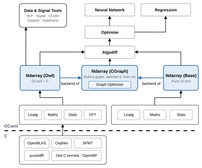
Owl is a rather complex library considering the numerous functions implemented (over 6500 functions by the end of 2020). We have strived for a modular design to make sure that the system is flexible enough to be extended in future. In the following, we will present its architecture briefly. Fig. 1.1 gives a bird’s-eye view of Owl’s numerical system architecture. From a perspective of numerical computing, the Owl modules can be categorised into three parts.
- The core modules are the foundation of computation. They mainly consist of the most basic data structures in Owl, namely the n-dimensional array, and the matrix. Besides, it also includes a foreign function interface to other libraries (e.g., CBLAS and LAPACKE).
- Based on the core modules, Owl provides modules that provide various classic analytics, including basic mathematical and statistical functions, linear algebra, signal processing, ordinary differential equations, etc. We will talk about them in Part I of this book.
- Furthermore, based on native support for algorithmic differentiation, Owl provides a series of advanced analytics, such as optimisation, regression, neural network, natural language processing, etc. Part II of this book includes these topics.
Owl provides two ndarray implementations with shared interfaces. The OCaml implementation, called Base, defines core data structures and numerical functions in pure OCaml. It provides a portable foundation, although some advanced operations are unavailable and its numerical kernels are generally slower than their C-backed counterparts.
The C-backed ndarray implementation combines OCaml with C numerical kernels and libraries, including CBLAS and LAPACKE. It provides the performance-oriented foundation for numerical computation on CPU.
A third form, CGraph-Ndarray, wraps either implementation to build computation graphs and support graph optimisation. These ndarray forms support higher-level modules such as algorithmic differentiation, optimisation and neural networks. Fig. 1.1 summarises these relationships, following Owl’s current code structure.1
There are other utility modules such as plotting. The separate owl-rllib library
builds on Owl to provide reinforcement learning algorithms and environments, as we
will see in Chap. 12.
Plotting is an indispensable function in modern numerical libraries. We build a
Plot module on top of PLplot [8] which is a powerful cross-platform plotting library.
However PLPlot only provides very low-level functions to interact with its multiple
plotting engines, even making a simple plot involves a very lengthy and tedious
control sequence. Using these low-level functions directly requires developers to
understand the mechanisms in depth. This can reduce productivity and make
mistakes more likely. Inspired by Matlab, we implement the Plot module to provide
developers a set of high-level APIs. The core plotting engine is very lightweight and
only contains about 200 lines of code. Its core design is to cache all the plotting
operations as a sequence of function closures and execute them all when we output
the figure. The figures in this book are mostly generated with the plotting
module, now provided by the separate owl-plplot package and opened as
Owl_plplot.
1.5 How to Run Code
“Always yield to the Hands-On Imperative.”
As a book on functional programming and scientific computing, this book contains a lot of code samples for the readers to run and explore by themselves. We encourage the readers to execute the given code first, and make some changes to better learn how it works.
We use matrixanger/springer-book-code, an Ubuntu-based Docker image, as
the reference environment. It contains the current stable OCaml compiler, Owl
main, the separately installed owl-plplot package, the numerical libraries,
and the dependencies used by the restored examples. Its exact compiler
version, upstream revisions and any recorded accuracy corrections are saved in
/opt/book/environment.json.
Use the validated latest image listed in the companion repository’s README;
its execution report states the chapter coverage. Refresh it and start a shell
with:
docker pull matrixanger/springer-book-code:latestdocker run --rm -it matrixanger/springer-book-code:latest bash
For a fixed edition, use its recorded image digest. Replace bash with utop for the
enhanced OCaml toplevel. Chapter commands run from /opt/book. The toplevel
loads Owl and plotting support. Each Running the examples box gives the source
directory and a command to run from a container shell. Source directory numbers are
stable identifiers and may differ from the printed chapter numbers; use the
directory given in the box. To follow the examples interactively, start a fresh
utop session, load the chapter setup, and work through the examples in
order. Longer setup listings appear next to the first example that needs
them.
All maintained example source belongs in the companion code repository, and the displayed excerpts and generated results are exported from it. Please check its README2 for the published image tags, detailed instructions, and records of source revisions, input checksums, numerical corrections and validation results.
1.6 Summary
This chapter briefly introduced the two key topics of this book, scientific computing and functional programming, before the main tool that is used in this book, the Owl library. It finished with an outline of the architecture of the Owl library, and how to run the code in this book.
Bibliography
- [1]
- Black-scholes model [Internet]. Wikipedia. Wikimedia Foundation; 2021
[cited 2022 Jan 4]. Available from:
https://en.wikipedia.org/wiki/Black-Scholes_model. - [2]
- McCarthy J. History of LISP. In: History of programming languages. 1978 Jun 1 (pp. 173-185).
- [3]
- Barendregt HP. The lambda calculus. Amsterdam: North-Holland; 1984.
- [4]
- Barendregt H, Manzonetto G, Plasmeijer R. The imperative and functional programming paradigm. In: Cooper SB, van Leeuwen J, editors. Alan Turing: His Work and Impact. Elsevier; 2013. pp. 121–126.
- [5]
- Turing AM. Computability and -definability. The Journal of Symbolic Logic. 1937 Dec;2(4):153-63.
- [6]
- Minsky, Y., Madhavapeddy, A., & Hickey, J. (2013). Real World OCaml: Functional programming for the masses. ” O’Reilly Media, Inc.”.
- [7]
- Monad (functional programming) [Internet].
Wikipedia. Wikimedia Foundation; 2022 [cited 2022 Jan 4]. Available from:
https://en.wikipedia.org/wiki/Monad_functional_programming. - [8]
- LeBrun MJ, Furnish G. The PLPLOT plotting library. Institute for Fusion Studies, University of Texas, Austin, USA. 2005.