CHAPTER 04
Linear Algebra
Linear algebra is an important area of mathematics and has many applications in numerical computing. In this chapter we first present an overview, and then focus on how to use OCaml to solve concrete problems and develop a thorough understanding of the key concepts in linear algebra. This chapter covers the classic topics in linear algebra, including Gaussian elimination, vector spaces, determinants, eigenvalues and eigenvectors. Before discussing these topics, we provide a brief introduction to the matrix data structure supported in OCaml.
4.1 Vectors and Matrices
Linear algebra is about solving systems of linear equations expressed in vectors
and matrices, hence we begin by familiarising ourselves with these basic elements.
The dense matrix functions can be accessed from the Dense.Matrix module, with
support for four number types: single, double, complex single, and complex double in
the Matrix.S, Matrix.D, Matrix.C and Matrix.Z modules respectively. The Mat
module is an alias of Matrix.D provided for convenience. Except for a handful of
functions (e.g., re to extract the real part of complex elements) most are
shared by these four sub-modules. Vectors can be represented as one-row or
one-column matrices. We will briefly discuss sparse matrix storage in the last
section.
There are multiple functions to help create matrices with certain contents. For
example, the following functions all create various 5x5 matrices:
Mat.empty 5 5, a matrix with uninitialised elementsMat.create 5 5 2., a matrix with all elements initialised to 2Mat.zeros 5 5, a matrix of all zerosMat.ones 5 5, a matrix of all onesMat.eye 5, an identity matrixMat.magic 5, a magic square matrixMat.uniform 5 5, a random matrix of uniform distributionMat.uniform_int 5 5, a random matrix with integer-valued elementsMat.sequential 5 5, a matrix of sequential integersMat.semidef 5, a random positive semidefinite matrixMat.gaussian 5 5, a random Gaussian matrixMat.bernoulli 5 5, a random Bernoulli matrix
In addition, to build a matrix from an OCaml array, use the of_array
operation, e.g., Mat.of_array [1.;2.;3.—] 1 3— builds a matrix of size
1x3.
The Mat module supports many mathematical operations on two matrices x and
y. For example, the matrix product Mat.dot x y can also be written Mat.(x *@ y),
and element-wise addition Mat.add x y can be Mat.(x + y). The approximate
element-wise equality comparison Mat.approx_equal can be used as Mat.(x =~ y).
Of course, these operations are all available for the other precisions, namely in the
Matrix.S/C/Z sub-modules.
If you perform operations between a matrix and a scalar value, you need to be careful
about their order. Assuming a is a float scalar value, we can add it to each element in
matrix
using Mat.(x +$ a) or Mat.(a $+ x). Note the difference between these
two operators, which have corresponding long names Mat.add_scalar and
Mat.scalar_add respectively.
There are other ready-made mathematical functions such as Mat.abs
(absolute value) and Mat.l2norm’, where the ’ in the name indicates that
the result is a scalar value rather than a 1x1 matrix. The matrix module
also contains operations such as concatenation (Mat.concat) and transpose
(Mat.transpose).
Finally, another key matrix operation is to index elements of the matrix,
supported via get and set to retrieve and modify elements by specifying zero-based
row and column indices, e.g.,
let x = Mat.uniform 5 5;;
Mat.set x 1 2 0.;;
let a = Mat.get x 0 3;;
The second line sets the element at (1,2) to 0, and then gets the value of the
element at (0,3). For dense matrices we can also use shorthand .%{i; j} to access
elements, rewriting the code above as:
Mat.(x.%{1;2} <- 0.);;
let a = Mat.(x.%{0;3});;
Matrix modifications using set are in-place.
We can retrieve rows from a matrix x by the rows function. The selected rows will
be used to assemble a new matrix. We can select columns similarly using
cols.
This section provides a very brief introduction to the matrix module and the
functions that will be used in the rest of this chapter. The matrix module builds on
the Ndarray (N-dimensional array) module, enabling matrices and ndarrays in Owl
to inter-operate. The Ndarray module and its functions, and thus the Matrix
module, are discussed in Chap. 5.
The rest of this chapter makes use of the Linalg module that provides various
high-level linear algebra APIs. As with the matrix module, it supports both real and
complex numbers in single and double precision. The Linalg.Generic module
provides the operations underlying Linalg.S/D/C/Z; some functions require explicit
output-type information. In this chapter, we will show how to use different aspects of
this module to investigate linear algebra topics.
4.2 Gaussian Elimination
Solving systems of linear equations is a core problem in linear algebra and is frequently encountered in scientific computation [1]. Gaussian Elimination is a classic method to do this, and it can work surprisingly well in modern numerical libraries [2]. Here is a simple example:
Divide the first equation by 2:
Multiply the first equation by -2 and add it to the second. Then multiply the first
equation by -3 and add it to the third. This gives us Eq. 4.3.
Finally, swapping the second and third, we get Eq. 4.4. We thus have , and can substitute for in the second equation to obtain . Plug both back to the first equation and we have .
This process demonstrated the basic operations of Gaussian elimination: eliminate unknown variables until the system of linear equations is easy to solve, and then back-substitute. There are three basic row operations we use: multiplying a row by a non-zero scalar, adding a multiple of one row to another, and swapping two rows. The starting equation Eq. 4.1 can be more concisely expressed with vectors:
or in the form using matrix notation:
Here is a matrix, is a column vector, and is the unknown vector we are solving for. Matrix notation is often used to describe systems of linear equations concisely.
4.2.1 LU Factorisation
Let’s look again at the Gaussian elimination example above. The final form Eq. 4.4 can be expressed with the matrix notation as:
As we can see, all the elements below the diagonal of the square matrix
are zero. Such a matrix is an upper triangular matrix, usually denoted
. Similarly, a
square matrix where all the elements above the diagonal are zero is a lower triangular matrix,
denoted .
We can use is_triu and is_tril in the Linalg module to test for
triangularity. In nonsingular square elimination, the diagonal entries of
are the pivots. The
-th pivot is the coefficient
used to eliminate the -th
variable at step ,
before any row normalisation.
When no row exchanges are needed, a square matrix can be factorised into a product of lower and upper triangular matrices:
| (4.5) |
and this process is called the LU factorisation. This embodies the process of Gaussian
elimination. Consider again the initial problem of solving the linear equation
.
One reason the LU factorisation is important is that if matrix
in
is
triangular, then solving it becomes straightforward, as seen in the previous example.
We can use the triangular_solve function in Linalg to efficiently solve the linear
equations if we already know that the matrix is triangular.
For a nonsingular square matrix with
, we can
change to
. First we find a
column vector
so that , then
we can find
so that .
Both sets of triangular equations are easy to solve. The lu function performs LU
factorisation with pivoting. Use the previous example once more:
# let a = [|
      2.;2.;2.;
      2.;2.;3.;
      3.;4.;5.;|];;
val a : float array = [|2.; 2.; 2.; 2.; 2.; 3.; 3.; 4.; 5.|]
# let a = Mat.of_array a 3 3;;
val a : Owl.Mat.mat =
   C0 C1 C2
R0  2  2  2
R1  2  2  3
R2  3  4  5
# let l, u, p = Linalg.D.lu a;;
val l : Owl.Linalg.D.mat =

         C0 C1 C2
R0        1  0  0
R1 0.666667  1  0
R2 0.666667  1  1

val u : Owl.Linalg.D.mat =

   C0        C1        C2
R0  3         4         5
R1  0 -0.666667 -0.333333
R2  0         0        -1

val p : Owl.Linalg.D.int32_mat =
   C0 C1 C2
R0  3  2  3
# let lu_pivots = p;;
val lu_pivots : Owl.Linalg.D.int32_mat =
   C0 C1 C2
R0  3  2  3
The first two returned matrices are the lower and upper triangular factors. However, if we multiply them without accounting for the pivoting, the result differs from the original matrix:
# let a' = Mat.dot l u;;
val a' : Owl.Mat.mat =
   C0 C1 C2
R0  3  4  5
R1  2  2  3
R2  2  2  2
It turns out that we need to account for row exchanges to obtain the correct answer. Pivoting avoids zero pivots where possible and, for numerical stability, may exchange rows even when a pivot is non-zero. This process is called pivoting. It is closely related to the stability of numerical computation. Choosing improper pivots can lead to incorrect solutions [3]. Pivoting can be expressed as a permutation matrix with the same rows as the identity matrix, each row and column having just a single element. The full LU factorisation can thus be expressed as:
# let p = Mat.of_array [|
      0.;0.;1.;
      0.;1.;0.;
      1.;0.;0.;
    |] 3 3;;
val p : Owl.Mat.mat =
   C0 C1 C2
R0  0  0  1
R1  0  1  0
R2  1  0  0
# Mat.(dot p a =~ dot l u);;
- : bool = true
Recall that the lu function also has a third output, the pivot
vector p, which contains the one-based LAPACK pivot indices
. We
save it as lu_pivots before reusing the name p for the manual permutation matrix.
How do we translate it to the previous permutation matrix? Each element
records the row
exchanged with row
at that elimination step. Subtract one from each pivot index for
OCaml’s zero-based indexing, and apply the row exchanges in forward
order to the identity matrix. This gives the permutation matrix
in
:
let perm_vec_to_mat vec =
  let n = Array.length vec in
  let permutation = Mat.eye n in
  Array.iteri (fun i pivot ->
    let j = pivot - 1 in
    if j < 0 || j >= n then invalid_arg "one-based LU pivot";
    for column = 0 to n - 1 do
      let value = Mat.get permutation i column in
      Mat.set permutation i column (Mat.get permutation j column);
      Mat.set permutation j column value
    done
  ) vec;
  permutation;;
let pivot_vector = Dense.Matrix.Generic.to_array lu_pivots
  |> Array.map Int32.to_int;;
let permutation = perm_vec_to_mat pivot_vector;;
Mat.(dot permutation a =~ dot l u);;
Note that there is more than one way to perform LU factorisation. For example, for the same matrix, a different pivot choice gives another factorisation:
4.2.2 Inverse and Transpose
The concept of an inverse matrix is related to the identity matrix
,
which is built via Mat.eye n where n is the size of the square matrix. The identity
matrix is a special form of Diagonal Matrix, a square matrix whose non-zero
elements occur only on its diagonal. We can check if a matrix is diagonal with the
is_diag function.
# Mat.eye 5 |> Linalg.D.is_diag;;
- : bool = true
The inverse of an square matrix is denoted as so that
| (4.6) |
Not all square matrices have inverses. There are many necessary and sufficient conditions that indicate if is invertible. One is that elimination produces non-zero pivots.
We use the function inv to perform matrix inversion. It is straightforward to verify the
result according to the definition. The example uses semidef, which generates a matrix of
the form .
Such a matrix is positive semidefinite, but is invertible only if
has
full column rank; the recorded sample is invertible.
# let x = Mat.semidef 5 in
    let y = Linalg.D.inv x in
    Mat.(x *@ y =~ eye 5);;
- : bool = true
Another frequently used operation is to take the transpose of a matrix. Denoted as , its -th row is taken from the -th column of the original matrix A. It has properties such as
| (4.7) |
We can verify this property using the matrix function Mat.transpose.
# let flag =
      let a = Mat.uniform 4 4 in
      let b = Mat.uniform 4 4 in
      let m1 = Mat.(dot a b |> transpose) in
      let m2 = Mat.(dot (transpose b) (transpose a)) in
      Mat.(m1 =~ m2);;
val flag : bool = true
Finally, a related special class of matrices is the Symmetric Matrix, those
matrices equal to their own transpose. This can be verified using the is_symmetric
function.
4.3 Vector Space
We have discussed solving the linear equations using Gaussian elimination where is a square matrix. We now discuss further how to determine whether there are any solutions and whether a solution is unique. To answer such questions, we need to be familiar with the concept of a vector space.
The vector space contains all column vectors with real elements. Its operations are vector addition and multiplication by real scalars. A linear combination is a sum of scalar multiples of vectors. A subspace is a non-empty subset closed under these operations: any linear combination of its vectors stays in the same subset.
There are four fundamental subspaces of interest when solving linear systems where is a real by matrix. The column space, a subspace of , is all linear combinations of the columns of . Similarly, the row space consists of all linear combinations of the rows of , viewed as vectors in . The nullspace contains all the vectors such that . It is a subspace of . The left nullspace is the nullspace of , a subspace of .
4.3.1 Rank and Basis
When discussing Gaussian elimination above, we assumed an ideal situation: matrix is an square matrix for which there exists a unique solution. But that is not always the case. may not even be a square matrix. When , a consistent system cannot have a unique solution; when , a system may be inconsistent. Besides, even when is a square matrix, the information contained in one equation might be repeated in another if, for example, one equation is simply a multiple of another. Applying Owl’s LU routine to the following singular matrix produces a failure:
# let x = Mat.of_array [|
    1.; 2.; 3.;
    0.; 0.; 1.;
    0.; 0.; 2.;
  |] 3 3;;
val x : Owl.Mat.mat =
   C0 C1 C2
R0  1  2  3
R1  0  0  1
R2  0  0  2
# let singular_lu_rejected =
    try ignore (Linalg.D.lu x); false
    with Failure _ -> true;;
val singular_lu_rejected : bool = true
This indicates a zero pivot in the second column. The matrix is singular, and this Owl call rejects it; the example catches that expected failure. A singular matrix may still have an LU factorisation, but its triangular factors cannot provide an invertible solve. As can be seen in this example, we cannot expect linear algebra functions to work without checking their assumptions.
To determine the solutions to a general
,
we must understand the concept of rank, the number of non-zero pivots
in row-echelon form. For a more intuitive understanding of rank, we
introduce the concept of linear independence. In a linear combination
where
are vectors
and are
scalars, if only
occurs when
for all ,
vectors
are linearly independent. The rank of a matrix is the maximum number of linearly
independent rows. We can understand rank as the number of “effective” rows in the
matrix. As an example, we can check the rank of the previous matrix with
Linalg.D.rank x. The result 2 indicates only two effective rows, so this
three-variable system cannot have a unique solution.
An application of rank produces a key concept in linear algebra: basis. A sequence of vectors is a basis of a vector space or subspace if the vectors are linearly independent, and all vectors in the space can be represented as a linear combination of vectors in the basis. A space can have infinitely many bases, but the number of vectors in each basis is the same and is called the dimension of the vector space. For example, if an matrix has rank , then the dimension of its null space is , and the dimension of its column space is . For a matrix with full column rank , its columns form a basis of its column space, and its null space has dimension zero, so the only solution of is the zero vector.
4.3.2 Orthogonality
We can relate the basis of a vector space to the Cartesian coordinate system in (for example) a three-dimensional space where every vector in the space can be represented in terms of values on the three axes, , and . There are many such basis sets but the set {, , } is convenient because all members are mutually orthogonal, simplifying many problems.
Orthogonality also applies to subspaces. Two real vectors and are orthogonal if , and we can say two subspaces and are orthogonal if every vector in is orthogonal to every vector in . For example, the nullspace and row space of a real matrix are orthogonal.
Among the bases of a subspace, one in which every vector is perpendicular to every
other is called an orthogonal basis. Moreover, if the length of each vector is normalised
to one unit, it is an orthonormal basis. A real square matrix whose columns form an
orthonormal basis is an orthogonal matrix. The null function returns a matrix
whose columns form an orthonormal basis for the null space, so
.
# let a = Mat.magic 4;;
val a : Owl.Mat.mat =

   C0 C1 C2 C3
R0  1 15 14  4
R1 12  6  7  9
R2  8 10 11  5
R3 13  3  2 16
# let x = Linalg.D.null a;;
val x : Owl.Linalg.D.mat =

          C0
R0 -0.223607
R1  -0.67082
R2   0.67082
R3  0.223607
# Mat.dot a x |> Mat.l2norm';;
- : Owl.Mat.elt = 4.48851511774729321e-15
Having defined orthogonal and orthonormal bases, how do
we build them? The QR Factorisation decomposes a real matrix
as
. For a reduced
factorisation with ,
has orthonormal columns
and is upper triangular;
if has full column
rank, the columns of
form a basis of its column space. It is provided in the linear algebra
module as the qr function, returning Q, R, and column pivot indices.
The default value of pivot is false, in which case the third result
is empty. Setting it to true performs a column-pivoted factorisation
, with
represented by one-based column indices.
# let a = Mat.of_array [|
      12.; -51.;   4.;
       6.; 167.; -68.;
      -4.;  24.; -41.;
    |] 3 3;;
val a : Owl.Mat.mat =

   C0  C1  C2
R0 12 -51   4
R1  6 167 -68
R2 -4  24 -41
# let q, r, _ = Linalg.D.qr a;;
val q : Owl.Linalg.D.mat =

          C0        C1         C2
R0 -0.857143  0.394286   0.331429
R1 -0.428571 -0.902857 -0.0342857
R2  0.285714 -0.171429   0.942857

val r : Owl.Linalg.D.mat =

    C0   C1  C2
R0 -14  -21  14
R1   0 -175  70
R2   0    0 -35
4.3.3 Solving Ax = b
We can now discuss the general solution structure of
and
where
is again an
matrix. There are non-zero
solutions to if and only if
the rank . The nullspace
then has dimension ,
and its
orthonormal basis vectors can be found with the null function. For example:
# let a = Mat.of_array [|
      1.; 5.;-1.;-1.;
      1.;-2.; 1.; 3.;
      3.; 8.;-1.; 1.;
      1.;-9.; 3.; 7.;
    |] 4 4;;
val a : Owl.Mat.mat =

   C0 C1 C2 C3
R0  1  5 -1 -1
R1  1 -2  1  3
R2  3  8 -1  1
R3  1 -9  3  7
# Linalg.D.rank a;;
- : int = 2
This is a rank 2 matrix, so the nullspace has dimension and the function returns two basis vectors:
# Linalg.D.null a;;
- : Owl.Linalg.D.mat =

          C0        C1
R0 -0.851419 0.0136382
R1  0.273706  0.143885
R2 0.0762491  0.962526
R3   0.44086 -0.229465
These two vectors form a fundamental system of solutions of . All solutions are their linear combinations; using the rounded coordinates displayed above, we write:
| (4.8) |
Here and can be any constant scalars. Considering the general form where is an vector, there exists just one solution if and only if where is a matrix formed by concatenating and along the column. If , has an infinite number of solutions with the general form:
| (4.9) |
where is a particular solution to , and form a basis of the nullspace, with . If , the system has no solution.
The function linsolve a b solves linear systems and least-squares problems of the
form .
By default, it uses LU factorisation with partial pivoting for a nonsingular square a.
For a rectangular full-rank matrix, it uses LAPACK’s QR or LQ least-squares solver.
The number of rows of a must equal the number of rows of b. For a square triangular
matrix, explicitly set typ:‘u or typ:‘l to select triangular_solve; the
default does not detect triangularity. The following matrix is rank deficient,
so we instead use its pseudoinverse to obtain a minimum-norm particular
solution.
# let a = Mat.of_array [|
       2.; 3.; 1.;
       1.;-2.; 4.;
       3.; 8.;-2.;
       4.;-1.; 9.;
    |] 4 3;;
val a : Owl.Mat.mat =

   C0 C1 C2
R0  2  3  1
R1  1 -2  4
R2  3  8 -2
R3  4 -1  9
# let b = Mat.of_array [|4.;-5.;13.;-6.|] 4 1;;
val b : Owl.Mat.mat =
   C0
R0  4
R1 -5
R2 13
R3 -6
# let x0 = Mat.dot (Linalg.D.pinv a) b;;
val x0 : Owl.Mat.mat =

          C0
R0  0.333333
R1   1.33333
R2 -0.666667
Then we use null to find a basis of the nullspace. You can verify that matrix a is of rank 2,
so the basis for
contains
vector.
# let x1 = Linalg.D.null a;;
val x1 : Owl.Linalg.D.mat =

          C0
R0 -0.816497
R1  0.408248
R2  0.408248
So the solutions to can be expressed as:
An important takeaway from this chapter is that using these functions in Linalg
requires a solid background in linear algebra. Blind application of them can easily
lead to wrong or misleading answers.
4.3.4 Matrix Sensitivity
The sensitivity of a linear system is crucial in numerical computation: in , how much can vary if we change or slightly? The Condition Number measures this sensitivity for a nonsingular square coefficient matrix [4].
First we need to understand the Norm, here the induced 2-norm of a real matrix , calculated as the square root of the maximum eigenvalue of . (The concept of eigenvalue will be introduced in Sec. 4.5.) This matrix norm gives an upper bound so that for any we have:
| (4.10) |
Here and
indicate the Euclidean
vector norm, and
denotes the induced 2-norm. It bounds how much
can amplify the input
; relative sensitivity
also involves .
We can calculate this matrix norm using Linalg.D.norm, whose default is
; it
differs from the Frobenius norm returned by Mat.l2norm’.
The most frequently used condition number is that representing
the sensitivity of inverse matrix [5]. Under the definition of norm,
the condition number for inversion of a matrix can be expressed as
, and
calculated using the cond function. Let’s look at an example:
# let a = Mat.of_array [|
      4.1; 2.8;
      9.7; 6.6;
    |] 2 2;;
val a : Owl.Mat.mat =
    C0  C1
R0 4.1 2.8
R1 9.7 6.6
# let c = Linalg.D.cond a;;
val c : float = 1622.99938385651058
Its condition number for inversion is much larger than one, so a small change in can lead to a large relative change in . Let’s look at one such perturbation.
# let a' = Linalg.D.inv a;;
val a' : Owl.Linalg.D.mat =
    C0  C1
R0 -66  28
R1  97 -41
Changing the last row of the matrix slightly and recalculating gives:
# let a2 = Mat.of_array [|
       4.1;   2.8;
      9.67; 6.607;
    |] 2 2;;
val a2 : Owl.Mat.mat =
     C0    C1
R0  4.1   2.8
R1 9.67 6.607
# let a2' = Linalg.D.inv a2;;
val a2' : Owl.Linalg.D.mat =

         C0       C1
R0  520.236 -220.472
R1 -761.417  322.835
As the large condition number warns, this small change to a causes a large change in its inverse.
The solution of
can also be sensitive, depending on the right-hand side and the perturbation.
4.4 Determinants
Besides pivots, another basic quantity in linear algebra is the determinant. An important application is to characterise whether a square matrix is invertible or singular. For an matrix, if and only if , i.e., is invertible. This is an exact-arithmetic statement; a floating-point determinant alone is not a reliable test for near-singularity.
For a square matrix :
its determinant is defined as:
The sum is over all permutations of . Here , where counts the indices for which . Mathematically, there are many techniques that can be used to simplify this calculation [6]. But as far as this book is concerned, it is sufficient for us to use the function to calculate the determinant of a matrix.
We can also use it to understand the solution of . If , has one and only one solution. This theorem is part of Cramer’s rule, and these properties are widely used when finding eigenvalues, discussed next.
When the determinant is positive and we need its logarithm, we can use logdet.
It sums logarithms of LU diagonal magnitudes rather than forming their product,
reducing the risk of overflow or underflow. The real-valued Owl routine rejects
negative determinants and singular inputs; it is not a general zero-determinant
test.
# let x = Mat.magic 5;;
val x : Owl.Mat.mat =

   C0 C1 C2 C3 C4
R0 17 24  1  8 15
R1 23  5  7 14 16
R2  4  6 13 20 22
R3 10 12 19 21  3
R4 11 18 25  2  9
# Linalg.D.det x;;
- : Owl.Linalg.D.elt = 5070000.
# Linalg.D.logdet x;;
- : Owl.Linalg.D.elt = 15.4388513755673671
4.5 Eigenvalues and Eigenvectors
In this section we move from studying to . The pattern
| (4.11) |
frequently appears in scientific and engineering analyses describing the change of a dynamic system over time [7]. For an square matrix, if there exists a scalar and a non-zero column vector satisfying:
| (4.12) |
then is an eigenvalue of , and is its corresponding eigenvector. To find the eigenvalues of a matrix , we must find the roots of the determinant of . is the characteristic equation of . For example, for matrix
Its characteristic matrix is:
By the definition of determinant, .
An -degree characteristic polynomial has complex roots counted with algebraic multiplicity. Specifically, here we have . Substituting into Eq. 4.12 gives . Therefore, we can find a basis for the nullspace of with:
# let basis =
      let ia = Mat.((eye 3) - (of_array
        [|3.; 1.;0.;
         -4.;-1.;0.;
          4.;-8.;2.|] 3 3))
      in
      Linalg.D.null ia;;
val basis : Owl.Linalg.D.mat =

           C0
R0 -0.0496904
R1  0.0993808
R2   0.993808
We thus get a fundamental solution .
Similarly, the eigenvectors for the eigenvalue are the non-zero scalar multiples of .
We can use the function eig to compute the right eigenvectors v and
eigenvalues w of an arbitrary square matrix x. The eigenvectors are column vectors
in v, their corresponding eigenvalues have the same order in w as that in
v.
# let eigvec, eigval =
      let a = Mat.of_array [|
          3.; 1.;0.;
         -4.;-1.;0.;
          4.;-8.;2.;
      |] 3 3 in
      Linalg.D.eig a;;
val eigvec : Owl.Linalg.D.complex_mat =

        C0               C1               C2
R0 (0, 0i)  (0.0496904, 0i)  (0.0496904, 0i)
R1 (0, 0i) (-0.0993808, 0i) (-0.0993808, 0i)
R2 (1, 0i)  (-0.993808, 0i)  (-0.993808, 0i)

val eigval : Owl.Linalg.D.complex_mat =

        C0      C1      C2
R0 (2, 0i) (1, 0i) (1, 0i)
Note that the results are expressed as complex numbers. To get just the
eigenvalues, we can use the eigvals function. Both functions take boolean arguments
permute and scale indicating whether the input matrix should be permuted or
diagonally scaled.
4.5.1 Complex Matrices
As in the previous examples, complex matrices are frequently used in calculating eigenvalues and eigenvectors, so we next re-introduce some concepts in complex spaces.
The notion of a symmetric matrix can be extended to the complex domain as the Hermitian
Matrix. A matrix
is Hermitian if ,
where
denotes its conjugate transpose: when transposing, each element
becomes its
complex conjugate .
The is_hermitian function tests if a matrix is Hermitian, as in the example
below.
# let a = Dense.Matrix.Z.of_array [|
      {re=1.; im=0.}; {re=2.; im=(-1.)};
      {re=2.; im=1.}; {re=3.; im=0.};
    |] 2 2;;
val a : Owl.Dense.Matrix.Z.mat =

        C0       C1
R0 (1, 0i) (2, -1i)
R1 (2, 1i)  (3, 0i)
# Linalg.Generic.is_hermitian a;;
- : bool = true
The conj function performs element-wise conjugation. Combining it with
transpose gives the conjugate transpose:
# Dense.Matrix.Z.(conj a |> transpose);;
- : Owl.Dense.Matrix.Z.mat =

         C0       C1
R0 (1, -0i) (2, -1i)
R1  (2, 1i) (3, -0i)
It can be shown that if a matrix is Hermitian, for all complex vectors , is real as are all its eigenvalues.
# Linalg.Z.eigvals a;;
- : Owl.Linalg.Z.complex_mat =

                         C0                      C1
R0 (-0.44949, 1.50231E-17i) (4.44949, 2.07021E-16i)
Related to the Hermitian matrix is the Unitary Matrix, a complex square matrix such that
| (4.13) |
The inverse and conjugate transpose of are equal; unitary matrices are the complex analogue of real orthogonal matrices.
4.5.2 Similarity Transformation and Diagonalisation
For an matrix , and an invertible matrix , the matrix
| (4.14) |
is said to be similar to , and has the same eigenvalues as . can be thought of as a matrix that changes basis while is a linear transformation, so first changes the basis before applying the linear transformation and changing the basis back. For example, in a three-dimensional space, may have three linearly independent vectors as its columns, expressed in the standard basis , , . Choosing a suitable basis can simplify the matrix representing the transformation. Finding a suitable similar matrix is thus key to simplifying calculations in many scientific and engineering problems.
One type of possible simplification is to find a triangular matrix that is
similar. The Schur decomposition theorem states that a complex square matrix
can be
written as ,
where is
unitary and
is upper triangular. A real Schur factorisation instead uses an
orthogonal matrix and an upper quasi-triangular matrix with
and
diagonal blocks. The complex decomposition can be computed using schur as
below:
# let a = Dense.Matrix.Z.of_array [|
      {re=1.; im=0.};    {re=1.; im=0.};
      {re=(-2.); im=0.}; {re=3.; im=0.};
    |] 2 2;;
val a : Owl.Dense.Matrix.Z.mat =

         C0      C1
R0  (1, 0i) (1, 0i)
R1 (-2, 0i) (3, 0i)
# let t, u, eigvals = Linalg.Z.schur a;;
val t : Owl.Linalg.Z.mat =

        C0                    C1
R0 (2, 1i) (2.10381, -0.757614i)
R1 (0, 0i)              (2, -1i)

val u : Owl.Linalg.Z.mat =

                       C0                      C1
R0 (-0.408248, 0.408248i)  (0.563384, -0.590987i)
R1        (-0.816497, 0i) (-0.577185, 0.0138014i)

val eigvals : Owl.Linalg.Z.complex_mat =

        C0       C1
R0 (2, 1i) (2, -1i)
The returned result t is upper triangular, and u is unitary, verified as
follows:
# Dense.Matrix.Z.(dot u (conj u |> transpose));;
- : Owl.Dense.Matrix.Z.mat =

                             C0                          C1
R0                      (1, 0i) (7.63278E-17, 3.38271E-17i)
R1 (7.63278E-17, -3.38271E-17i)                     (1, 0i)
Another very important similarity transformation is diagonalisation. Suppose has linearly independent eigenvectors that are the columns of a matrix , then is a diagonal matrix , and the eigenvalues of are the diagonal elements of . Equivalently,
| (4.15) |
is the Eigen Decomposition. Analysing ’s diagonal similar matrix rather than directly often greatly simplifies problems.
Note that not every matrix can be diagonalised. If none of the eigenvalues of are equal, then corresponding eigenvectors are linearly independent and can be diagonalised over the complex numbers. In particular, every real symmetric matrix can be diagonalised by an orthogonal matrix, and every Hermitian matrix by a unitary matrix.
4.6 Positive Definite Matrices
We now introduce the Positive Definite Matrix, unifying the three key ideas introduced so far: pivots, determinants, and eigenvalues.
4.6.1 Positive Definiteness
A real matrix is Positive Definite if it is symmetric and
| (4.16) |
for all non-zero vectors . There are several necessary and sufficient conditions that can be used to test if a symmetric matrix is positive definite:
- for all non-zero real vectors x;
- for all eigenvalues of A;
- all leading principal submatrices have positive determinants;
- all the pivots without row exchange satisfy ;
- there exists an invertible real matrix such that .
For the last condition, we can use the Cholesky Decomposition to find the matrix
.
A Hermitian positive definite matrix has a factorisation
with
lower
triangular, or
with
upper triangular. Owl’s chol returns the upper factor by default. Although
named l in the example below, the result is upper triangular and satisfies
for
this real input:
# let a = Mat.of_array [|
       4.; 12.;-16.;
      12.; 37.;-43.;
     -16.;-43.; 98.;
     |] 3 3;;
val a : Owl.Mat.mat =

    C0  C1  C2
R0   4  12 -16
R1  12  37 -43
R2 -16 -43  98
# let l = Linalg.D.chol a;;
val l : Owl.Linalg.D.mat =

   C0 C1 C2
R0  2  6 -8
R1  0  1  5
R2  0  0  3
# Mat.(dot (transpose l) l =~ a);;
- : bool = true
If we know that
in
is Hermitian and positive definite, we can solve
using the default
upper factor, or
when requesting upper:false. As we have seen previously, solving triangular systems
is easy. For such matrices, Cholesky factorisation requires fewer operations than
general LU factorisation. In Linalg, is_posdef checks whether Cholesky
factorisation succeeds. The input must already be known to be symmetric or
Hermitian: the routine uses one triangle and does not independently check
symmetry.
# Linalg.D.is_posdef a;;
- : bool = true
The definition of positive semidefinite is similar: is real symmetric and for all real vectors . The following Eq. 4.17 exists in many engineering analyses.
| (4.17) |
If and are real symmetric positive definite, the generalised eigenvalues are positive. Eigenvalues also appear in the study of the continuous-time linear system , where
We will see how to compute a Jacobian matrix in Chap. 8. In a system linearised about an equilibrium, is the Jacobian evaluated there. For the linear system , asymptotic stability requires all eigenvalues of to have strictly negative real parts; positive eigenvalues instead imply growth. A symmetric positive definite matrix for which is positive semidefinite guarantees Lyapunov stability. If is positive definite, it guarantees asymptotic stability [13].
4.6.2 Singular Value Decomposition
The singular value decomposition (SVD) is one of the most important matrix factorisations. It provides a numerically stable matrix decomposition that is both useful for many purposes and guaranteed to exist [8]. Specifically, any real matrix can be factorised as:
| (4.20) |
Here is an orthogonal matrix whose columns are eigenvectors of . Similarly, is an orthogonal matrix whose columns are eigenvectors of . If has rank , the rectangular diagonal matrix has positive singular values, the square roots of the non-zero eigenvalues of and ; its remaining diagonal entries are zero. SVD is thus related to the eigendecompositions of these positive semidefinite matrices. For a real symmetric positive definite matrix , the eigendecomposition also gives an SVD.
Looking more closely, Eq. 4.20 can be expressed as Eq. 4.21. Here and are column vectors of length and respectively. Each is an rank-one matrix. Therefore, SVD expresses as a sum of such matrices, each scaled by its singular value, ordered . The larger the singular value is, the more weight is given to its corresponding matrix. If a singular value is small, omitting that term introduces an error of magnitude in the induced 2-norm. This is a fundamental use of SVD: it can locate the “significant” components in a matrix, and is thus often used to reduce the dimension of given data.
| (4.21) |
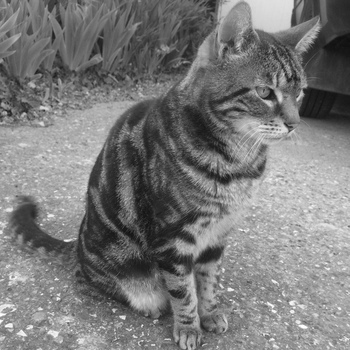
As an example, we will now demonstrate how to use SVD to re-encode an image using less information, i.e. image compression. We will use
a cat image as shown in Fig. 4.1a. First, we load the image as a matrix using the code below.
#use "imageUtils.ml";;
module N = Dense.Ndarray.S;;
module M = Dense.Matrix.S;;
let img_arr = load_ppm "cat_bw.ppm" |> N.get_slice [[];[];[0]];;
let shp = N.shape img_arr;;
let h, w = shp.(0), shp.(1);;
let img = N.reshape img_arr [|h; w|];;
The output img is a
matrix of floating-point values initially representing integer pixel intensities between
0 and 255 in this greyscale image. For simplicity, we don’t use external image
libraries, but use the image-related utility functions in imageUtils.ml provided in
the code repository of this book. It provides routines to handle the PPM image
format. After obtaining img, we can apply SVD to it. The SVD is supported in the
Linalg module.
# let u, s, vt = Linalg.S.svd img;;
val s : Owl.Linalg.S.mat =

        C0      C1      C2         C347     C348     C349
R0 43899.6 7480.73 4876.87 ... 0.960703 0.694049 0.324325
The output is three matrices representing
, the singular
values, and ;
only the singular-value vector is displayed above. Both u and vt are
matrices. The
diagonal entries of
are returned in the row vector s, sorted from large to small. We
can form a square diagonal matrix using M.diagm s, where M is the
Dense.Matrix.S alias used here. By default Owl returns a reduced SVD with
singular
values, an
matrix ,
and a
matrix , so
this square
diagonal factor also works for rectangular inputs.
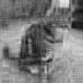
Next we reconstruct the image using the first
singular values. For
example, let’s set ,
a relatively small value. That means we need to set every element in s to zero except
for the first 10, which we do by using a slicing method. You may be familiar with
such array manipulation techniques from systems such as NumPy. If not, don’t worry
– we will explain in detail in Chap. 5.
let l = (N.shape s).(1);;
let n = 10;;
let s' = N.copy s;;
let z = N.zeros [|1; l - n|];;
let _ = N.set_slice [[];[n; l - 1]] s' z;;
The new
diagonal values are contained in s’. We can now reconstruct the original image matrix by
calculating :
let img' = M.(dot (dot u (diagm s')) vt);;
The resulting matrix img’ can be saved in PPM format using our customised
image save routine in imageUtils.ml.
let image = N.stack ~axis:2 [|img'; img'; img'|];;
let image = N.expand image 4;;
let fname = "cat_" ^ (string_of_int n) ^ ".ppm";;
let _ = save_ppm_from_arr image fname;;
The reconstructed figure is shown in Fig. 4.1b. Even though it has lost a lot of detail, it nonetheless provides a sketch of the original image. For the original matrix, we need to store values. Using SVD, each and contains 350 elements, while is a scalar. To reconstruct the approximation we only need to keep the first 10 , , and , storing values, about 5.7% of the original value count. This compares numbers of values, not bytes: the original pixels and floating-point factors use different storage formats.
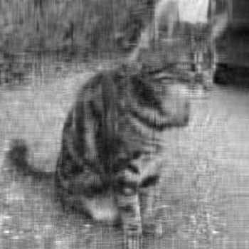
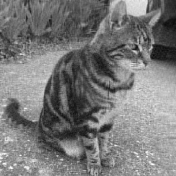
While retaining far fewer values, the reconstructed image is clearly of quite low quality. We can improve it by keeping more singular values, setting (Fig. 4.1c) and (Fig. 4.1d). By the time we use 50 components, requiring about 28.6% of the original value count, the reconstructed figure is already quite close to the original.
Besides svd, the Linalg module also provides several variants such as
svdvals returning the singular values, and gsvd performing a generalised
SVD where gsvd x y -> (u, v, q, d1, d2, r) computes the generalised
SVD of a pair of general rectangular matrices x and y. Here d1 and d2
contain the generalised singular value pairs of x and y. The shape of x is
and the
shape of y is .
SVD has a wide and growing range of applications [9] [10]. The
example above uses a low-rank image representation, demonstrating its
application in dimensionality reduction. The reconstructed image still has
pixels, but is represented using only 10, 20, or 50 singular components. Similarly,
SVD can compress other high-dimensional data to simplify processing. In Chap. 13
we will see how truncated SVD reduces the dimension of a document-term
representation in language processing; PCA uses SVD of centred data. The
Moore-Penrose pseudo-inverse, which also applies to non-invertible and rectangular
matrices, can be computed using SVD, and Owl provides Linalg.D.pinv for
this [11].
4.7 Sparse Matrices
What we have discussed so far is based on dense matrices. But often non-zero
elements are sparsely distributed, as in the identity matrix. A sparse structure can
save storage and computation by avoiding explicit zero elements. The Sparse.Matrix
interface described in the first edition is not exported by the Owl version in the
reference environment. In this final section, we introduce sparse storage formats
without assuming that interface is available.
The most intuitive method to represent a matrix is the (row, column, value)
triplet where, using zero-based indices as in Owl, (1,2,10) means that the element
in the second row and third column is 10. Tuples can be sorted according to row and
column values to improve access efficiency.
Another commonly used format is the Compressed Sparse Row (CSR) format which is similar to the triplet above but compresses row indices. For example, suppose we must represent the following matrix:
The CSR format retains the column indices and values but replaces repeated row indices with row pointers. The triplets on the right of Fig. 4.2 store six row indices. The left shows the three row starts ; a complete CSR row-pointer array also includes the terminal offset 6, giving . Each row uses the segment between two successive pointers in the value and column-index arrays. Entries in a row need not share a column index.
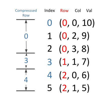
Using this representation, one can quickly locate a given element in the sparse
matrix. For example, to search the (2, 1, 5) triplet, we know that we can search
this element from the index 4 by checking the compressed row indices, and then look
for the column number 1. The benefit of CSR is that it is more efficient at accessing
row-vectors and performing row operations. Another data structure Compressed
Sparse Column (CSC) is similar but compresses column vectors instead of
rows.
Triplets are an intuitive format for constructing a sparse matrix: new entries can be appended before sorting and combining duplicates. CSR and CSC provide efficient row and column access respectively, as well as arithmetic such as matrix-vector multiplication. Changing the sparsity pattern can be expensive, though updating an existing stored value need not be. Eigen, an optimised C++ library for linear algebra, implements variants of these storage schemes 1.
4.8 Summary
This chapter gave an overview of several important topics of Linear Algebra. Starting from basic vector and matrix operations, we briefly introduced several key ideas from this field, including Gaussian elimination, vector spaces, determinants, Eigenvalues, Positive Definite Matrices, etc. We demonstrated these topics with examples and code using Owl. We closed with a discussion of the sparse matrix and its representation formats used.
Bibliography
- [1]
- Oliphant TE. Python for scientific computing. Computing in science & engineering. 2007 Jun 18;9(3):10-20.
- [2]
- Baboulin M, Buttari A, Dongarra J, Kurzak J, Langou J, Langou J, Luszczek P, Tomov S. Accelerating scientific computations with mixed precision algorithms. Computer Physics Communications. 2009 Dec 1; 180(12):2526-33.
- [3]
- Skeel RD. Iterative refinement implies numerical stability for Gaussian elimination. Mathematics of computation. 1980; 35(151):817-32.
- [4]
- Zames G. Feedback and optimal sensitivity: Model reference transformations, multiplicative seminorms, and approximate inverses. IEEE Transactions on automatic control. 1981 Apr; 26(2):301-20.
- [5]
- Lorber A. Error propagation and figures of merit for quantification by solving matrix equations. Analytical Chemistry. 1986 May 1; 58(6):1167-72.
- [6]
- MacDonald JKL. Successive approximations by the Rayleigh-Ritz variation method. Physical Review. 1933 May 15; 43(10):830.
- [7]
- Fox RL, Kapoor MP. Rates of change of eigenvalues and eigenvectors. AIAA journal. 1968 Dec; 6(12):2426-9.
- [8]
- Stewart GW. On the early history of the singular value decomposition. SIAM review. 1993 Dec; 35(4):551-66.
- [9]
- Andrews H, Patterson C. Singular value decompositions and digital image processing. IEEE Transactions on Acoustics, Speech, and Signal Processing. 1976 Feb; 24(1):26-53.
- [10]
- Maciejewski AA, Klein CA. The singular value decomposition: Computation and applications to robotics. The International journal of robotics research. 1989 Dec; 8(6):63-79.
- [11]
- Biglieri E, Yao K. Some properties of singular value decomposition and their applications to digital signal processing. Signal Processing. 1989 Nov 1; 18(3):277-89.
- [12]
- Strang G. Linear Algebra and Its Applications. 3rd ed. San Diego: Harcourt Brace Jovanovich; 1988.
- [13]
- Cross GW. Three types of matrix stability. Linear algebra and its applications. 1978 Jun 1; 20(3):253-63.