CHAPTER 06
Ordinary Differential Equations
A differential equation is an equation that contains a function and one or more of its derivatives. They have been studied ever since the invention of calculus, driven by applications in fields including mechanics [1], astronomy [2], geometry, biology [3], engineering [4], economics [5], and many more. If the unknown function depends on one independent variable, we call it an Ordinary Differential Equation (ODE). A system of ODEs can describe several state variables evolving with time. A Partial Differential Equation (PDE) involves partial derivatives of a function of several independent variables. In this chapter we focus on ODEs, including their definition, numerical solution, and the tools provided by Owl.
6.1 Defining an ODE
In general an ordinary differential equation can be expressed as:
| (6.1) |
This relates an unknown function to its derivatives. ODEs can be used to model dynamical systems. For an initial value problem of order , the initial values specify the function and its first derivatives at the same point :
| (6.2) |
where the , , etc. are known. The highest order of derivatives occurring in Eq. 6.1 is the order of the differential equation. A first-order differential equation in explicit form can be expressed as:
| (6.3) |
where is a given function of and . Solving Eq. 6.1 and fitting to the given initial values as in Eq. 6.2 is called the initial value problem. Solving such problems is the main target of many numerical ODE solvers.
6.1.1 Exact Solutions
Many differential equations cannot be solved analytically and we must turn to numerical solvers to make progress. However, before doing so let us first look at some ODEs that do have analytical closed-form solutions.
Tbl. 6.1 shows two examples. The first row gives a separable equation, while the second gives a linear first-order equation. Their solutions are given in the second column. Here is a constant determined by the initial condition , and . In the first row, depends on ; in the second, depends on . In both rows depends on . The derivative can be isolated as a function of and (where in the first row), giving an explicit ODE, in contrast to an implicit ODE.
Higher order ODEs in explicit form can be reduced to systems of first-order ODEs by introducing additional state variables. For example, an ODE in the form can be reduced by multiple integrations on both sides. If a second-order ODE is in the form , let , so that . Substitution gives , a first-order ODE. If we can solve it to obtain , then integration gives .
Please refer to classical calculus books or courses for more detail on the analytical solution of ODEs. We turn now to methods for their numerical solution.
6.1.2 Linear Systems
ODEs are often used to describe various dynamic systems. In the previous
examples there is only one function, y, that changes over time. However, a real world
system often contains multiple interdependent components, each described by
a function that evolves over time. Later we will talk about several ODE
examples in detail, including the two-body problem and the Lorenz attractor. For
now we simply observe that Eq. 6.12 and Eq. 6.13 in the sections below
are quite different from the ODE forms above. For example, the Lorenz
attractor system has three components that change with time: the rate of
convection in the atmospheric flow, the horizontal and vertical temperature
variation.
Both are first-order systems of ODEs, but both are nonlinear. A linear system of ODEs is a special case in which the derivatives depend linearly on the state variables. If we have:
then a linear system can be expressed as:
| (6.4) |
This linear system contains time-dependent components: . The numerical solvers used here accept first-order systems, which need not be linear. Transforming a higher order single-component ODE into such a system is therefore often necessary, as we will see in the two-body problem example. But let’s get back to the start and examine the basics of solving ODEs numerically.
6.2 Solving ODEs Numerically
This section introduces the basic idea of solving the initial value problem numerically. Let’s start with an example:
| (6.5) |
where the initial value is . This is a separable first-order ODE, and according to Tbl. 6.1,
its analytical closed-form solution is shown in Eq. 6.6.
| (6.6) |
However, imagine we don’t have the solution but want to know the value of when (or any other value). How can we solve it numerically?
Enter Euler Method, a first-order numerical procedure to solve initial value problems. The basic idea is simple: from Eq. 6.5 we know the derivative, or the “slope” at any given point on the function curve, and we know the initial value and of this function. We can then simply move from the initial point to the target value in small steps, adjusting the direction according to the derivative at every new point. Formally, the Euler method proposes to approximate the function using a sequence of iterative steps:
| (6.7) |
where is a certain step size. This method is easy to implement in OCaml, as shown below.
let x = ref 0.;;
let y = ref 0.;;
let target = 1.;;
let step = 0.001;;
let f x y = 2. *. x *. y +. x;;
while !x < target do
  let h = min step (target -. !x) in
  y := !y +. h *. (f !x !y);
  x := !x +. h
done;;
In this case, we know that the analytical solution at is :
# (Owl_const.e -. 1.)/. 2.;;
- : float = 0.859140914229522545
and the numerical result approaches this value as the step size decreases.
However, although this method is easy and works well in this example, its low order of accuracy and restrictive stability conditions can require very small steps. This simple implementation also provides no error estimate. However, we can modify Euler’s method to use a “midpoint” when making steps in an attempt to curb the error in the update process as below.
The method then becomes the Midpoint Method. Let’s compare the performance of Euler and Midpoint in approximating the true result in Eq. 6.6:
let f x y = 2. *. x *. y +. x
let f' x = 0.5 *. (Maths.exp (x *. x) -. 1.)

let integrate advance step target =
  if not (Float.is_finite step && step > 0. && Float.is_finite target && target >= 0.)
  then invalid_arg "finite positive step and nonnegative target required";
  let steps = int_of_float (ceil (target /. step)) in
  let y = ref 0. in
  for i = 0 to steps - 1 do
    let x = float_of_int i *. step in
    let h = min step (target -. x) in
    y := advance x !y h
  done;
  !y

let euler step target =
  integrate (fun x y h -> y +. h *. f x y) step target

let midpoint step target =
  integrate (fun x y h ->
    let slope = f x y in
    y +. h *. f (x +. h /. 2.) (y +. h *. slope /. 2.)
  ) step target;;
let _ =
  let target = 2.6 in
  let h = Plot.create "plot_rk01.png" in
  Plot.(plot_fun ~h ~spec:[ RGB (66,133,244); LineStyle 1;
    LineWidth 2.; Marker "*" ] f' 2. target);
  Plot.(plot_fun ~h ~spec:[ RGB (219,68,55); LineStyle 2;
    LineWidth 2.; Marker "+" ] (euler 0.01) 2. target);
  Plot.(plot_fun ~h ~spec:[ RGB (219,68,55); LineStyle 2;
    LineWidth 2.; Marker "." ] (euler 0.001) 2. target);
  Plot.(plot_fun ~h ~spec:[ RGB (244,180,0); LineStyle 3;
    LineWidth 2.; Marker "+" ] (midpoint 0.01) 2. target);
  Plot.(plot_fun ~h ~spec:[ RGB (244,180,0); LineStyle 3;
    LineWidth 2.; Marker "." ] (midpoint 0.001) 2. target);
  Plot.(legend_on h ~position:NorthWest
    [|"Close-Form Solution"; "Euler (step = 0.01)";
    "Euler (step = 0.001)"; "Midpoint (step = 0.01)";
    "Midpoint (step = 0.001)"|]);
  Plot.output h;;
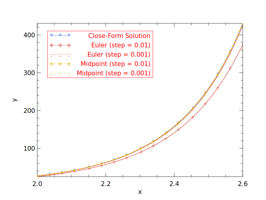
Fig. 6.1 shows that the choice of step size indeed matters to accuracy. We use 0.01 and 0.001 for step size in the test, and for both cases the Midpoint method outperforms the simple Euler method.
But why stop at only one midpoint? We can continue this process and add further intermediate stages in the update sequence seeking to improve accuracy further. For example, we can do this:
In this method, each iteration computes four intermediate steps: at the initial point, at the end, and twice at the midpoints. The resulting method is often more accurate than the midpoint method.
We can continue like this but hopefully you can see the pattern now. In fact, these seemingly magical parameters are related to the terms in Taylor series expansions. In previous methods, e.g. Euler method, every time you update to , an error is introduced into the approximation. A method of order matches the Taylor expansion through , giving a local error of order and, under suitable smoothness and stability assumptions, a global error of order . This family of methods is called the Runge-Kutta Methods, where the basic idea is to remove the errors order by order, using the correct set of coefficients [6]. For sufficiently small steps and smooth solutions, higher order can give smaller error.
Euler’s method is the most basic Runge-Kutta (RK) method, while the Midpoint
method is also called the second-order Runge-Kutta Method (rk2). What Eq. 6.8 shows
is a fourth-order Runge-Kutta method (rk4). It is a widely used RK method, and works
surprisingly well in many cases. It is often a good choice especially when computing
is not
expensive [7] [8].
However, as powerful as it may be, the classical rk4 used here still has a fixed
step size and no built-in error estimate. Adaptive Runge–Kutta solvers add error
estimation and update the step size rather than holding it constant. Other methods
also exist such as the Adams-Bashforth Method and Backward Differentiation
Formula (BDF), both multi-step methods that use more information than just the
derivative of the current step to compute the solution at next step, such as
values from previous time steps [9]. The Bulirsch-Stoer method is another
established approach that can be accurate and efficient for smooth, non-stiff
problems. Discussion of these advanced numerical methods and techniques is
beyond the scope of this book. Please refer to Numerical Recipes [10] for more
information.
6.3 ODE Solvers
In practice we obviously do not want to reimplement these manual calculations
every time. It’s time to introduce some tools. Built on the computational
functionality and ndarray data structures already introduced, the package owl-ode
performs the tasks of solving the initial value problems [18].
6.3.1 Solving a Linear System
We will use a simple linear system example to demonstrate how to use the
owl-ode package to solve ODE problems. More practical and interesting examples
will be shown in Sec. 6.4.
Consider the following time-independent linear dynamical system of two states:
This system has real eigenvalues , so it describes growth and decay rather than oscillation. Here is the state of the system, is time, and the initial state at is . We wish to know the system state at . The function can be expressed in Owl using the matrix module.
let f y t =
  let a = [|[|1.; -1.|];[|2.; -3.|]|]|> Mat.of_arrays in
  Mat.(a *@ y);;
Next, we want to specify the timespan of this problem: from 0 to 2 using a step of 0.001.
let tspec = Owl_ode.Types.
  (T1 {t0 = 0.; duration = 2.; dt=1E-3});;
The last requirement for solving the problem is to have the initial values:
let x0 = Mat.of_array [|-1.; 1.|] 2 1;;
Finally we pass these parameters to the rk4 solver in Owl_ode. The result contains the sample times
and the corresponding
system states :
# let ts, ys = Owl_ode.Ode.odeint
    Owl_ode.Native.D.rk4 f x0 tspec ();;
val ts : Owl_ode.Native.D.mat =

   C0    C1    C2     C1998 C1999 C2000
R0  0 0.001 0.002 ... 1.998 1.999     2

val ys : Owl_ode.Native.D.mat =

   C0       C1       C2        C1998    C1999    C2000
R0 -1   -1.002 -1.00399 ...   -3.566 -3.56749 -3.56898
R1  1 0.995005 0.990022 ... -2.07617 -2.07707 -2.07798
6.3.2 Solver Structure
From this example, we can see that owl-ode abstracts the
initial value problems as four different parts: (1) a function
to show how the system
evolves in equation ;
(2) a specification of the timespan; (3) a set of system’s initial values; and most
importantly, (4) a solver.
Indeed, the signature of a solver clearly indicates these four parts:
val rk4 :
  (module Owl_ode.Native.D.Types.Solver with type f = Owl_ode.Native.D.mat ->
                                                      float ->
                                                      Owl_ode.Native.D.mat and type solve_output =
   Owl_ode.Native.D.mat * Owl_ode.Native.D.mat and type state = Owl_ode.Native.D.mat and type step_output =
   Owl_ode.Native.D.mat * float)
Building on this uniform abstraction, a user can choose a suitable solver and use it to solve many complex and practical ODE problems. Note that due to the difference of solvers, the requirements of different solvers vary, e.g., some require the state to be two matrices, while others process data using a more general ndarray format.
Owl-ode provides a wide range of solvers. It implements native solvers based on
the basic step-by-step update idea discussed above, and also interfaces to external
libraries. The reference container uses the native solvers and the LSODA solver from
ODEPACK1.
SUNDIALS2 is another numerical solver library with optional OCaml bindings. Those bindings are not part of the reference OCaml 5 environment. The examples below use native RK45 for non-stiff problems and ODEPACK’s LSODA for the stiff example. Tbl. 6.2 lists the native and ODEPACK solvers; symplectic solvers are discussed next.
These solvers share similar signatures. The system evolution function takes state
y and time t as input and returns the derivative of y. The solver returns
two matrices or ndarrays containing the sample times and corresponding
states.
For many non-stiff problems, rk45 is a reasonable first solver to try because it
estimates local error and adapts its step size. Other native solvers may be useful
when a fixed time grid is needed or less accuracy is sufficient; efficiency
depends on the problem and the requested accuracy. For stiff problems, a solver
designed for that purpose is needed; the ODEPACK LSODA backend is used
later in this chapter. We will talk about the stiffness of ODEs in a later
section.
6.3.3 Symplectic Solver
In addition to the above, owl-ode also implements symplectic solvers, which
preserve the geometric structure of Hamiltonian dynamics [11]. This can improve
long-term behaviour without necessarily giving higher pointwise accuracy. We will
illustrate the motivation with an example.
Consider a simple harmonic oscillator. Its position and velocity trace a circle in phase space when we solve the normalised linear system:
| (6.9) |
This can also be expressed in matrix form as:
| (6.10) |
We can then apply the previous methods such as Euler to solve it:
let f y t =
  let a = [|[|0.; 1.|];[|-1.; 0.|]|]|> Mat.of_arrays in
  Mat.(a *@ y);;
let x0 = Mat.of_array [|1.; 0.|] 2 1;;
let tspec = Owl_ode.Types.(
  T1 {t0 = 0.; duration = 10.; dt=1E-2});;
let ts, ys = Owl_ode.Ode.odeint
  Owl_ode.Native.D.euler f x0 tspec ();;
let _ =
  let h = Plot.create "plot_circle.png" in
  Plot.plot ~h (Mat.row ys 0) (Mat.row ys 1);
  Plot.output h;;
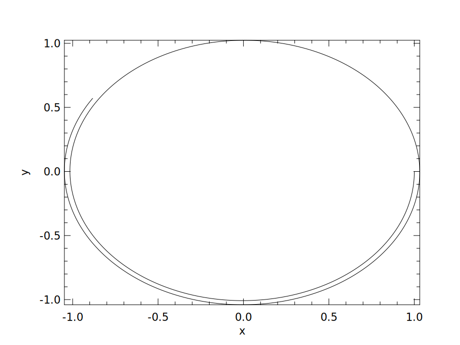
To see the resulting trajectory, we plot the two components of ys in Fig. 6.2. An
exact solution would generate a perfect circle, but here we obtain a spiral (the step
size here is 0.01; the outward drift persists for any positive fixed step size). Aside
from using a more accurate solver, are there any other ways we could improve this
solution?
Look again at Eq. 6.9. Setting and , we have and . This is a Hamiltonian system, a class often used in classical mechanics. Such systems are represented by coordinates , where the ’s are the generalised coordinates and the ’s the corresponding conjugate momenta. The evolution of a Hamiltonian system is defined by:
Here is the Hamiltonian; in the example above, is the energy. Symplectic solvers preserve phase-space geometry, not generally the exact value of . For suitable Hamiltonian problems and step sizes, their energy error can remain small over long times.
Most of the numerical solvers we mentioned above, including the Euler and classical RK solvers, are not symplectic solvers.
Owl_ode has implemented several symplectic solvers based on different integration
algorithms: symplectic_euler, leapfrog, pseudoleapfrog, ruth3, and
ruth4 in Symplectic.D. Like native solvers, they have different orders of
accuracy on the Hamiltonian problems for which they are designed. The
implementations use different update sequences and coefficients. If you are interested
in more detail, please check the code and the paper of Candy et al. [12] on
which the implementation is based. Later in this chapter we will show an
example of using this solver interface for a damped harmonic oscillator, where
damping means that the usual symplectic conservation properties no longer
apply.
6.3.4 Features and Limits
One feature of owl-ode is the automatic inference of state dimensionality from
the initial state. For example, the native solvers take an input matrix as the
state. Suppose the initial state of the system is a row vector of dimension
. For
recorded
times, including the initial time, the states are stacked vertically and have shape
.
If the initial state is a column vector of shape
, the trajectory
instead has shape .
The temporal integration of matrices, i.e. cases where the initial state is a
matrix instead of a vector, is also supported. For an initial state of shape
, with both
dimensions greater than one, the native solvers return a three-dimensional ndarray of shape
. If this trajectory is
explicitly reshaped to ,
the helper Native.D.to_state_array (N,M) can unpack it into an array of
matrices.
Another feature of owl-ode is that users can configure a solver with different
parameters while keeping the same odeint interface. For example, we create a native
RK45 solver with tol=1E-7 and dtmax=0.1:
let custom_rk45 = Owl_ode.Native.D.rk45
  ~tol:1E-7 ~dtmax:0.1;;
let ts, xs = Owl_ode.Ode.odeint custom_rk45 f x0 tspec ();;
Here, rk45 constructs a configured first-class solver module. The tol
parameter controls the local error threshold. In the version used by this
book, dtmax limits the next step suggested by the module’s low-level step
function; odeint instead sets its own maximum step to the integration interval
divided by 128. These are not the separate relative and absolute tolerances of
CVODE.
The owl-ode aims to run across different backends such as JavaScript. One way
to do this is to use tools like js_of_ocaml to convert OCaml bytecode into
JavaScript. However, external C or Fortran dependencies need separate JavaScript
implementations or bindings. The SUNDIALS and ODEPACK backends therefore
cannot simply be compiled this way. The owl-ode-base package contains solver
algorithms written in OCaml; these can be used in a browser with a compatible
numerical backend.
6.4 Examples of ODE Solvers
As with many good things, mastering ODE solution requires a lot of practice.
After getting to know owl-ode, in this section we will demonstrate more examples of
using this tool.
6.4.1 Explicit ODE
For a starter, now we can use owl-ode to solve the motivating problem in Eq. 6.5
with some straightforward code.
let f y t = Mat.((2. $* y *$ t) +$ t);;
let tspec = Owl_ode.Types.(
  T1 {t0 = 0.; duration = 1.; dt=1E-3});;
let y0 = Mat.zeros 1 1;;
let solver = Owl_ode.Native.D.rk45 ~tol:1E-9 ~dtmax:10.0;;
let _, ys = Owl_ode.Ode.odeint solver f y0 tspec ();;
The code is quite similar to the previous example, except that we can now try
another provided solver, the rk45 solver, with certain parameters specified. The roles
of tol and dtmax are described in Sect. 6.3.4.
The result is shown below. You can verify the result with Eq. 6.6, by setting to 1 in this equation, and the numerical value of will be close to 0.859141.
# Mat.transpose ys;;
- : Owl.Mat.mat =

   C0          C1         C2         C127     C128     C129
R0  0 1.90735E-06 4.7686E-05 ... 0.822728 0.843353 0.859141
6.4.2 Two-body Problem
In classical mechanics, the two-body problem is to predict the motion of two massive objects. We assume that the objects interact only with each other. This problem appears in astrodynamics, where planets and satellites move under mutual gravitation.
This classic problem is one of the earliest investigated mechanics problems, and has been studied since Newton. With inverse-square gravitational attraction, it is an integrable problem in classical mechanics. In this example, let’s consider a simplified version of this problem. We assume that the two objects interact on a 2-dimensional plane, and one of them is so much more massive than the other one that it can be thought of as being static (think about a planet and the Sun), sitting at the origin of a Cartesian coordinate system in the plane. In this system, let’s consider the trajectory of the lighter object. This “one-body” problem is the basis of the two body problem. More generally, an isolated two-body problem with a central force separates into free centre-of-mass motion and a relative-motion problem with a reduced mass.
Given the previous assumption and Newton’s equations, it can be proved3 that the location of the lighter object [, ] with regard to time can be described by:
| (6.11) |
where , and units are chosen so that the gravitational parameter is one. This is a second-order ODE system, and so to make it solvable using our tool we must transform it into a first-order explicit ordinary differential equation system:
Based on Eq. 6.12, we can build up our code as below:
let f y _t =
  let y = Mat.to_array y in
  let r = Maths.(sqrt ((sqr y.(0)) +. (sqr y.(1)))) in
  let y0' = y.(2) in
  let y1' = y.(3) in
  let y2' = -.y.(0) /. (Maths.pow r 3.) in
  let y3' = -.y.(1) /. (Maths.pow r 3.) in
  [| [|y0'; y1'; y2'; y3'|] |] |> Mat.of_arrays;;

let y0 = Mat.of_array [|-1.; 0.; 0.5; 0.5|] 1 4;;

let tspec = Owl_ode.Types.(T1 {
  t0 = 0.;
  duration = 20.;
  dt=1E-2});;

let custom_solver = Native.D.rk45 ~tol:1E-9 ~dtmax:10.0;;
Here y0 provides the initial state of the system: the first two numbers denote the
initial location of the object, and the next two indicate the initial velocity of the
object. After building the function, initial state, timespan, and solver, we can then
solve the system and visualise it with the code below. The result is shown in
Fig. 6.3.
let plot () =
  let ts, ys = Ode.odeint custom_solver f y0 tspec () in
  let h = Plot.create "two_body.png" in
  let open Plot in
  plot ~h ~spec:[ RGB (66, 133, 244); LineStyle 1 ]
    (Mat.col ys 0) (Mat.col ys 1);
  scatter ~h ~spec:[ Marker "#[0x229a]"; MarkerSize 5. ]
    (Mat.zeros 1 1) (Mat.zeros 1 1);
  text ~h ~spec:[ RGB (51,51,51)] (-.0.3) 0. "Massive Object";
  output h;;
plot ();;
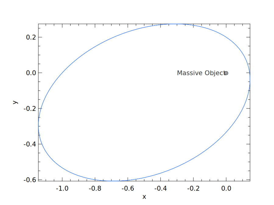
An example of this simplified two-body problem is the “planet-sun” system where a planet orbits the sun. Kepler’s first law states that a bound planetary orbit is an ellipse, with the Sun at one focus. The orbiting trajectory in the result visually follows this theory.
6.4.3 Lorenz Attractor
The Lorenz equations form one of the most thoroughly studied systems of ODEs. Edward Lorenz proposed this simplified model of thermal convection in 1963 [13]. The model reduces the convection equations to the three equations below.
Here is proportional to the rate of convection in the atmospheric flow; and are proportional to the temperature difference between ascending and descending currents and the departure of the vertical temperature profile from linearity, respectively. Parameter is the Prandtl number [14], and is the normalised Rayleigh number. is related to the geometry of the domain. The parameter setting used here is , and .
Based on this information, we can use owl-ode to express the Lorenz equations
with code.
let sigma = 10.;;
let beta = 8. /. 3.;;
let rho = 28.;;
let f y _t =
  let y = Mat.to_array y in
  let y0' = sigma *. (y.(1) -. y.(0)) in
  let y1' = y.(0) *. (rho -. y.(2)) -. y.(1) in
  let y2' = y.(0) *. y.(1) -. beta *. y.(2) in
  [| [|y0'; y1'; y2'|] |] |> Mat.of_arrays;;
Now, we can solve the ODE system and visualise the results. In Fig. 6.4, we first show how the values of , and change with time; next we show the pairwise phase-space projections.
let y0 = Mat.of_array [|-1.;0.;0.5|] 1 3;;
let _ =
  let ts, ys = Ode.odeint custom_solver f y0 tspec () in
  let h = Plot.create ~m:2 ~n:2 "lorenz_01.png" in
  let open Plot in
  subplot h 0 0;
  set_xlabel h "time";
  set_ylabel h "value on three axes";
  plot ~h ~spec:[ RGB (66, 133, 244); LineStyle 1 ] ts (Mat.col ys 2);
  plot ~h ~spec:[ RGB (219, 68,  55); LineStyle 1 ] ts (Mat.col ys 1);
  plot ~h ~spec:[ RGB (244, 180,  0); LineStyle 1 ] ts (Mat.col ys 0);
  subplot h 0 1;
  set_xlabel h "x-axis";
  set_ylabel h "y-axis";
  plot ~h ~spec:[ RGB (66, 133, 244) ] (Mat.col ys 0) (Mat.col ys 1);
  subplot h 1 0;
  set_xlabel h "y-axis";
  set_ylabel h "z-axis";
  plot ~h ~spec:[ RGB (66, 133, 244) ] (Mat.col ys 1) (Mat.col ys 2);
  subplot h 1 1;
  set_xlabel h "x-axis";
  set_ylabel h "z-axis";
  plot ~h ~spec:[ RGB (66, 133, 244) ] (Mat.col ys 0) (Mat.col ys 2);
  output h;;
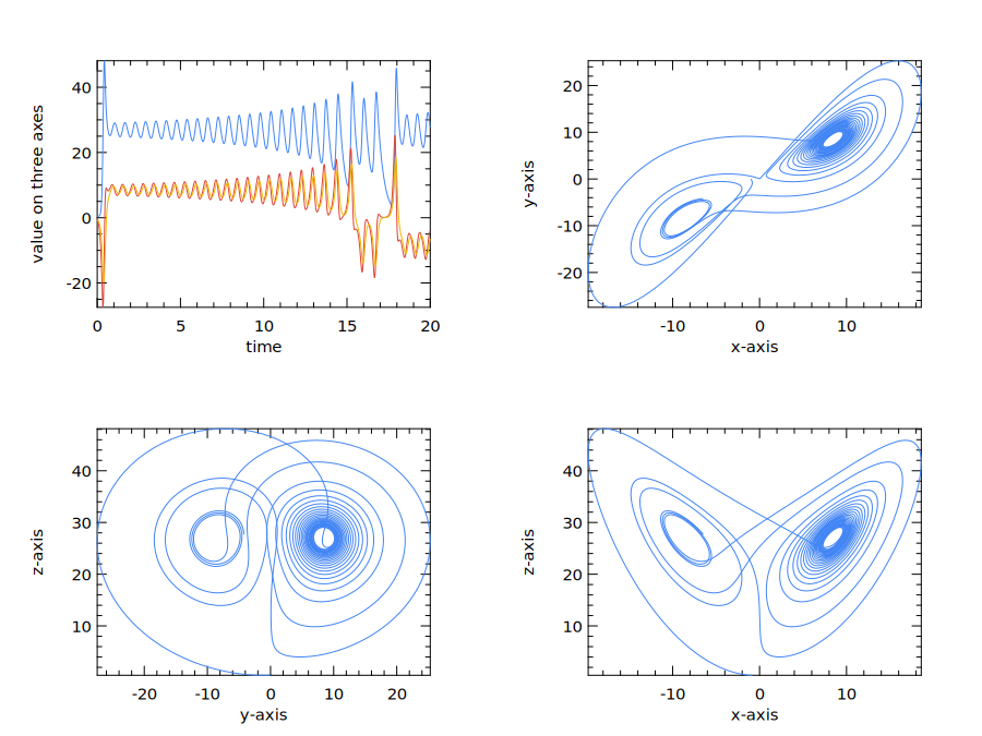
From Fig. 6.4, we can imagine the trajectory winding around one lobe in three-dimensional space before moving to the other. The trajectory winds around two lobes of a single attractor in this dynamical system; the two empty centres are not themselves attractors.
When considering the Lorenz equation, an interesting question is “what would happen if I change the initial value slightly?” For some systems, such as a simple undamped harmonic oscillator, a small initial change remains small, but not here. We can see that clearly with a simple experiment. Keeping function and timespan the same, let’s change the initial value by just 0.1% and then solve the system again.
let comparison_solver = Native.D.rk4;;
let y00 = Mat.of_array [|-1.; -1.; 1.|] 1 3;;
let y01 = Mat.of_array [|-1.001; -1.001; 1.001|] 1 3;;
let ts0, ys0 = Ode.odeint comparison_solver f y00 tspec ();;
let ts1, ys1 = Ode.odeint comparison_solver f y01 tspec ();;
For this comparison we use the same fixed-step RK4 solver for both initial states. This gives a common physical time grid; simply truncating two adaptive trajectories to the same length would not align their observation times. We check that the times and shapes agree before comparing the states.
assert (Mat.shape ts0 = Mat.shape ts1 && Mat.approx_equal ts0 ts1);;
let ts = ts0;;
assert (Mat.shape ys0 = Mat.shape ys1);;
Now, we can compare the Euclidean distance between the states of these two systems at each recorded time. We also show how the three components of the perturbed trajectory change over time.
let _ =
  let h = Plot.create ~m:1 ~n:2 "lorenz_02.png" in
  let open Plot in
  subplot h 0 0;
  set_xlabel h "time";
  set_ylabel h "value on three axes";
  plot ~h ~spec:[ RGB (244, 180,  0); LineStyle 1 ] ts (Mat.col ys1 0);
  plot ~h ~spec:[ RGB (219, 68,  55); LineStyle 1 ] ts (Mat.col ys1 1);
  plot ~h ~spec:[ RGB (66, 133, 244); LineStyle 1 ] ts (Mat.col ys1 2);
  subplot h 0 1;
  let diff = Mat.(
    sqr ((col ys0 0) - (col ys1 0)) +
    sqr ((col ys0 1) - (col ys1 1)) +
    sqr ((col ys0 2) - (col ys1 2))
    |> sqrt
  )
  in
  plot ~h ~spec:[ RGB (66, 133, 244); LineStyle 1 ] ts diff;
  set_xlabel h "time";
  set_ylabel h "distance of two systems";
  output h;;
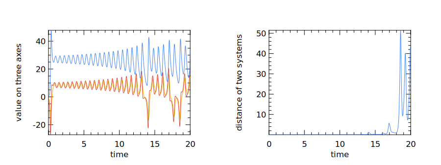
In Fig. 6.5, the right-hand plot shows that the initially nearby trajectories eventually separate substantially. The distance fluctuates rather than growing monotonically or without bound. The left-hand plot shows the perturbed trajectory; Fig. 6.4 uses a different initial state, so it is not the unperturbed reference for this comparison. For these parameter values, even a tiny change in the initial state can lead to a large difference in the future state after a while. This partly explains why weather prediction is difficult to do: you can only accurately predict the weather for a certain period of time; any farther into the future and the weather will be extremely sensitive to a tiny bit of perturbations at the beginning. As the pop culture reference has it, perhaps even the flapping of the wings of a distant butterfly several weeks earlier could be enough.
6.4.4 Damped Oscillation
Damped oscillation ODE systems appear frequently in physics and many other fields, including charge flow in electric circuits [15], sound waves [16], light waves [17], etc. One simple example is a mass attached to a vertical spring. The spring initially stretches to balance gravity; once the system reaches equilibrium, we can then study the upward displacement of the mass from its equilibrium position, . Once the mass is in motion, at any position , the net restoring force on the mass is proportional to displacement , where is a positive parameter.
This system is called a simple harmonic oscillator, representing an ideal case where is the only force acting on the mass. However, in a real physical system there will also be friction, giving rise to damped oscillation. For linear viscous damping, the frictional force is proportional and opposite to the velocity of the mass and so the total force can be expressed as where is the damping coefficient factor. Using Newton’s second law, we have, for the mass of the object:
| (6.14) |
Recall from the previous section that the state of the system in a symplectic solver is a tuple of two matrices, representing the position and momentum coordinates of the system. We can use the same interface to express the damped oscillation equation. Damping makes this a dissipative system: its mechanical energy decreases, so the usual Hamiltonian symplectic guarantees do not apply to this example.
let a = 1.0;;
let damped_noforcing a (xs, ps) _t : Owl.Mat.mat =
  Owl.Mat.((xs *$ -1.0) + (ps *$ (-1.0 *. a)));;
The system evolution function damped_noforcing takes the two
matrices, position and momentum, and the float number time t as input
states.4
It returns the force, or equivalently the rate of change of momentum. For simplicity, we
set ,
so momentum equals velocity numerically. Let’s then solve with the symplectic solver
and compare the Leapfrog, ruth3, and Symplectic_Euler:
let main () =
  let x0 = Owl.Mat.of_array [| -0.25 |] 1 1 in
  let p0 = Owl.Mat.of_array [| 0.75 |] 1 1 in
  let t0, duration = 0.0, 15.0 in
  let f = damped_noforcing a in
  let tspec = T1 { t0; duration; dt=0.1 } in
  let t, sol1, _ = Ode.odeint (module Symplectic.D.Leapfrog)
    f (x0, p0) tspec () in
  let _, sol2, _ = Ode.odeint Symplectic.D.ruth3
    f (x0, p0) tspec () in
  let _, sol3, _ =
    Ode.odeint (module Symplectic.D.Symplectic_Euler)
    f (x0, p0) tspec ()
  in
  t, sol1, sol2, sol3;;
Hopefully this code is not too surprising now: it first defines the initial values, the time duration, time step, and then provides this information to the solvers. Unlike the native solvers discussed earlier, these solvers return three values instead of two. The first is the time sequence, and the next two sequences indicate how the and values evolve at each time point.
let plot_sol fname t sol1 sol2 sol3 =
  let h = Plot.create fname in
  let open Plot in
  plot ~h ~spec:[RGB (0,0,255); LineStyle 1] t (Mat.col sol1 0);
  plot ~h ~spec:[RGB (0,150,0); LineStyle 2] t (Mat.col sol2 0);
  plot ~h ~spec:[RGB (200,0,0); LineStyle 3] t (Mat.col sol3 0);
  legend_on h [| "Leapfrog"; "Ruth3"; "Symplectic Euler" |];
  output h;;
let t, sol1, sol2, sol3 = main ();;
plot_sol "damped.png" t sol1 sol2 sol3;;
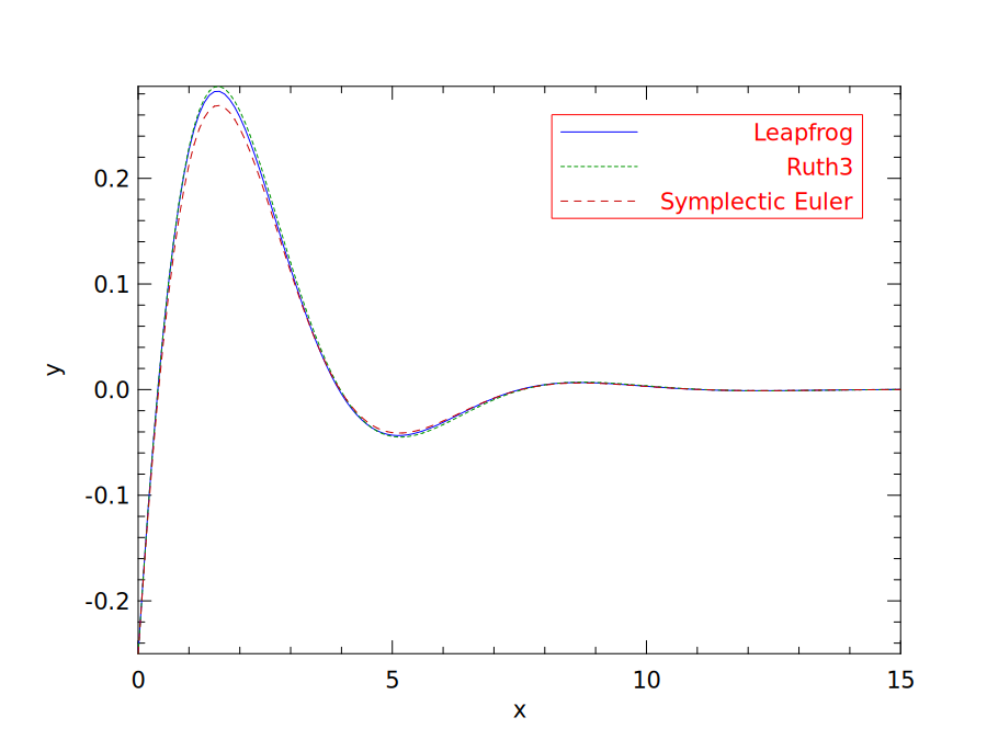
Here we only plot the change of position over time in the oscillation, and the solution provided by the three different solvers, as shown in the plotting code above. You can also try to visualise the change to the momentum in a similar way. The result is shown in Fig. 6.6. You can clearly see that the oscillation amplitude decreases towards the equilibrium position in this damped oscillation as the energy of the system dissipates. The curves provided by three solvers are a bit different, especially at the peak of the curve, but are reasonably close most of the time.
6.5 Stiffness
Stiffness is an important concept in the numerical solution of ODEs. In a stiff problem, stability can force an explicit solver to take much smaller steps than accuracy alone requires, even where the solution is smooth. Covering the whole timespan can then take a very long time. Methods designed for stiff problems, often implicit methods, can avoid this severe stability restriction; adaptive step size alone does not remove it [19].
The Van der Pol equation is a good example to show both non-stiff and stiff cases. In dynamics, the Van der Pol oscillator is a non-conservative oscillator with non-linear damping [20]. Its behaviour with time can be described with a second-order ODE:
| (6.15) |
where is a scalar parameter controlling the non-linearity and the strength of the damping. To make it solvable using our tool, we rewrite it as a pair of explicit first-order ODEs in a nonlinear system:
| (6.16) |
As we will show shortly, by varying the damping parameter this group of equations can be made either non-stiff or stiff.
We use native RK45 for the non-stiff case and ODEPACK LSODA, which can switch between stiff and non-stiff algorithms, for the stiff case. Both start with the same differential equations:
open Owl_ode;;
open Owl_ode.Types;;
open Owl_plplot;;

let van_der_pol mu =
  fun y _t ->
    let y = Mat.to_array y in
    let a = y.(1) in
    let b = mu *. (1. -. Maths.sqr y.(0)) *. y.(1) -. y.(0) in
    [|[|a; b|]|] |> Mat.of_arrays;;
6.5.1 Solving Non-Stiff ODEs
When , the equation is non-stiff. We solve it with native RK45, keeping the initial state and 30-unit time interval:
let f_non_stiff = van_der_pol 1.;;
let y0 = Mat.of_array [| 0.02; 0.03 |] 1 2;;
let tspec = T1 { t0 = 0.0; dt = 0.01; duration = 30.0 };;
let ts, ys = Ode.odeint (Native.D.rk45 ~tol:1E-8 ~dtmax:0.05)
  f_non_stiff y0 tspec ();;
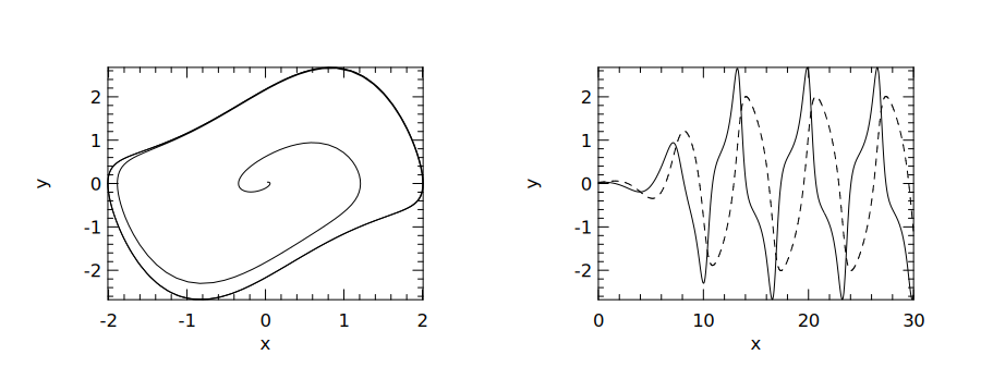
We can plot how the two state components change over time, together with their
trajectory in the phase plane, using the two components as the axis values. The
result is shown in Fig. 6.7.
let () =
  let fname = "vdp_rk45_nonstiff.png" in
  let h = Plot.create ~n:2 ~m:1 fname in
  let open Plot in
  subplot h 0 0;
  plot ~h ~spec:[ LineStyle 1 ] (Mat.col ys 0) (Mat.col ys 1);
  subplot h 0 1;
  plot ~h ~spec:[ LineStyle 1 ] ts Mat.(col ys 1);
  plot ~h ~spec:[ LineStyle 3 ] ts Mat.(col ys 0);
  output h;;
6.5.2 Solving Stiff ODEs
However, changing the parameter to
makes this problem stiff . We follow the same procedure as before, but now we use
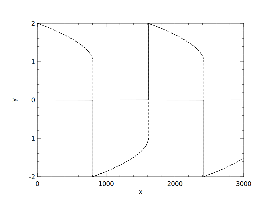
the lsoda solver from ODEPACK and extend the timespan to 3000. Fig. 6.8 shows
rapid transitions separated by much slower evolution. This separation of time scales
is characteristic of this stiff example; a sharp-looking curve alone is not a test for
stiffness.
let f_stiff = van_der_pol 1000.;;
let y0 = Mat.of_array [| 2.; 0. |] 1 2;;
let tspec = T1 { t0 = 0.0; dt = 0.01; duration = 3000.0 };;
let () =
  let ts, ys = Ode.odeint (module Owl_ode_odepack.Lsoda)
    f_stiff y0 tspec () in
  let fname = "vdp_odepack_stiff.png" in
  let h = Plot.create fname in
  let open Plot in
  set_yrange h (-2.) 2.;
  plot ~h ~spec:[ LineStyle 1 ] ts Mat.(col ys 1);
  plot ~h ~spec:[ LineStyle 3 ] ts Mat.(col ys 0);
  output h;;
6.6 Summary
This chapter discussed numerical solutions to the initial value problem for
ordinary differential equations (ODEs). We presented the general definition of the
ODE and the initial value problem. We explained how the numerical solutions are
developed. Then we presented owl-ode, an OCaml library that solves ODEs based on
Owl. Besides implementing native solvers, it also interfaces to external solver
libraries; the examples here use native solvers and ODEPACK. We demonstrated how
these solvers are used to solve ODEs from several real examples, including the
two-body problem, the Lorenz Attractor, and Damped Oscillation. Finally, we briefly
discussed an important concept: stiffness, when solving ODEs numerically, and
showed how we can solve stiff and non-stiff ODEs with the example of the van der
Pol equation.
Bibliography
- [1]
- Dirac PA. On the theory of quantum mechanics. Proceedings of the Royal Society of London. Series A, Containing Papers of a Mathematical and Physical Character. 1926 Oct 1;112(762):661-77.
- [2]
- Chandrasekhar S. Stochastic problems in physics and astronomy. Reviews of modern physics. 1943 Jan 1;15(1):1.
- [3]
- Agarwal P, Deniz S, Jain S, Alderremy AA, Aly S. A new analysis of a partial differential equation arising in biology and population genetics via semi analytical techniques. Physica A: Statistical Mechanics and its Applications. 2020 Mar 15;542:122769.
- [4]
- Zhang B, Zhang T, Cao Z, Zhang K. Fast new small-target detection algorithm based on a modified partial differential equation in infrared clutter. Optical engineering. 2007 Oct;46(10):106401.
- [5]
- Boucekkine R, Fabbri G, Pintus P. On the optimal control of a linear neutral differential equation arising in economics. Optimal Control Applications and Methods. 2012 Sep;33(5):511-30.
- [6]
- Hairer E, Nørsett SP, Wanner G. Solving Ordinary Differential
Equations I: Nonstiff Problems [Internet]. Springer Berlin Heidelberg;
2008. Springer Series in Computational Mathematics. Available from:
https://books.google.com.sg/books?id=F93u7VcSRyYC. - [7]
- Carpenter MH, Kennedy CA, Bijl H, Viken SA, Vatsa VN. Fourth-order Runge-Kutta schemes for fluid mechanics applications. Journal of Scientific Computing. 2005 Nov; 25(1):157-94.
- [8]
- Hult J. A fourth-order Runge-Kutta in the interaction picture method for simulating supercontinuum generation in optical fibers. Journal of Lightwave Technology. 2007 Dec 1;25(12):3770-5.
- [9]
- Butcher JC. Numerical methods for ordinary differential equations. John Wiley & Sons; 2016 Aug 29.
- [10]
- Press WH, Teukolsky SA, Vetterling WT, Flannery BP. Numerical recipes 3rd edition: The art of scientific computing. Cambridge University Press; 2007 Sep 6.
- [11]
- Yoshida H. Construction of higher order symplectic integrators. Physics letters A. 1990 Nov 12;150(5-7):262-8.
- [12]
- Candy J, Rozmus W. A symplectic integration algorithm for separable Hamiltonian functions. Journal of Computational Physics. 1991 Jan 1; 92(1):230-56.
- [13]
- Lorenz EN. Deterministic nonperiodic flow. Journal of the Atmospheric
Sciences. 1963;20(2):130–141.
2.0.CO;2" class="url" >
https://doi.org/10.1175/1520-0469(1963)020<0130:DNF>2.0.CO;2. - [14]
- White FM. Viscous fluid flow. 3rd ed. McGraw-Hill; 2006.
- [15]
- Zhang R. Computational Science and Engineering I, Week
5 lecture notes, Sect. 5.1. MIT OpenCourseWare; 2020.
https://ocw.mit.edu/courses/18-085-computational-science-and-engineering-i-summer-2020/resources/mit18_085summer20_lec_w5/. - [16]
- Sprague MW. The single sonic muscle twitch model for the sound-production mechanism in the weakfish, Cynoscion regalis. The Journal of the Acoustical Society of America. 2000 Nov; 108(5):2430-7.
- [17]
- Haken H. Cooperative phenomena in systems far from thermal equilibrium and in nonphysical systems. Reviews of modern physics. 1975 Jan 1; 47(1):67.
- [18]
- Seri M, Kao TC. OwlDE: making ODEs first-class Owl citizens. Journal of Open Source Software. 2019 Dec 20;4(44):1812.
- [19]
- Petzold L. Automatic selection of methods for solving stiff and nonstiff systems of ordinary differential equations. SIAM journal on scientific and statistical computing. 1983 Mar;4(1):136-48.
- [20]
- Van der Pol B. On “relaxation-oscillations”. The London, Edinburgh, and
Dublin Philosophical Magazine and Journal of Science.
1926;2(11):978–992.
https://doi.org/10.1080/14786442608564127.