CHAPTER 18
Case Study: Autonomous Driving
A camera image, a short question and a few numbers are enough to give us an interesting programming problem: how can one model describe a driving scene and predict where the car should go? We follow an OCaml implementation of SimLingo from its inputs to its answer and waypoints. Small array examples introduce attention, the merging of image patches, the assembly of a multimodal sequence and the accumulation of predicted displacements. We then read the corresponding model code, including its vision encoder, language generation loop and driving heads. The chapter ends by running the model on recorded scenes and examining its outputs.
18.1 A Driving Scene
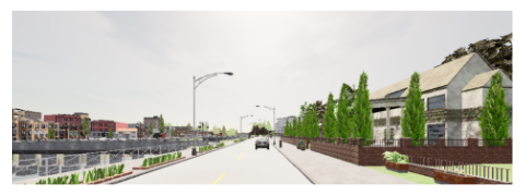
Imagine that we are sitting in the car whose camera produced Fig. 18.1. A car is travelling ahead of us. Our current speed is 9.5 metres per second, and the planned route continues along the road. We ask a program, “What should the ego do next?” Here, ego means the car carrying the camera. The program replies:
Follow the route. Maintain the reduced speed to stay behind
the black car that is to the front in 24.7 meters. Waypoints:
Alongside the sentence, the program returns two arrays of coordinates. The first contains 20 points describing a route; the second contains 10 points describing future positions at successive times. A waypoint is a position through which a planned path passes. In this chapter, coordinates are measured in metres relative to the car: the first coordinate points forward, and the second points to its right. The car is at . Thus means ten metres ahead and one metre to the left.
The two arrays answer related questions. The route describes the shape of the path ahead. Its training targets were sampled at one-metre intervals, starting at the origin and extending to 19 metres along the path. The speed waypoints describe where the car should be after 0.25, 0.50, and so on up to 2.50 seconds. Their spacing therefore also conveys speed. We will return to this distinction when we read the output heads. Here are the first few coordinates from our example:
Route: first three of 20 points (m)
  (  0.001,   0.005)
  (  0.999,   0.025)
  (  1.999,   0.048)
Speed waypoints: first three of 10 points (m)
  (  2.412,   0.093)
  (  4.814,   0.077)
  (  7.179,   0.028)
Generated tokens, including EOS: 31
eos_reached: true
The input also contains two target points, approximately and . These are navigation instructions supplied to the model. Keep them separate from the waypoints that the model predicts. The target points tell it where the route is heading; the output waypoints describe its proposed motion in the scene. The program receives the recorded coordinates at their original precision. We round them here to make their meaning easier to see.
Our task is to understand the computation behind these results. We will use
SimLingo, a model that combines camera-based driving with language [2]. Its
trained parameters are already available. We will load them and perform inference:
compute an output for a new input while keeping those parameters fixed. The
implementation lives in the companion repository’s simlingo-owl/ directory. Its
numerical operations use Owl.Dense.Ndarray.S, which stores single-precision arrays.
The arrays and neural-network operations from Chaps. 5 and 11 remain useful here: matrices, slices, dot products, activation functions and loops. What changes is their arrangement. We shall follow one frame through that arrangement, pausing at four short OCaml examples where a small array makes a large model easier to understand.
18.2 The SimLingo Pipeline
The phrase vision–language–action, often shortened to VLA, names the three parts of our task. Vision supplies information about the visible scene. Language supplies the question and the answer. Action supplies a numerical description of the intended movement. Figure 18.2 shows how these parts meet in the implementation.
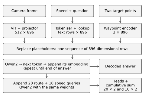
The first branch turns the camera image into a sequence of vectors. A vision Transformer processes small image regions and combines information between them. A projection then gives each resulting vector 896 components. We will see why the branch produces exactly 512 such vectors for our frame.
The second branch prepares the text. A tokenizer divides text into units called tokens, each identified by an integer. A token may represent a word, part of a word, punctuation or a special marker. The model looks up each integer in a table of learned vectors. This lookup gives an embedding: the numerical row with which the model represents that token. These rows also have 896 components.
The third branch takes the two navigation target points through a small neural network. Each pair of coordinates becomes another 896-component row. At the junction of the branches, image and target rows replace designated placeholders in the text sequence. The result is one two-dimensional array. Its first dimension counts positions in the sequence; its second dimension counts features at each position.
A language Transformer then updates this array. The implementation uses the Qwen2 language component of the InternVL2-1B model on which this SimLingo checkpoint is built [5, 6]. From the last updated row, it computes scores for possible next tokens and selects one. It appends the selected token’s embedding and repeats. Once the answer ends, the program appends 30 learned vectors, called driving queries. Twenty request route points; ten request speed waypoints. One more pass through the language Transformer supplies their output states. Two small networks turn those states into coordinate displacements, which are accumulated into positions.
We can keep the code map short. Preprocess prepares pixels; Vit encodes the image; Tokenizer prepares
text; and Qwen2 updates the combined sequence. Simlingo assembles these operations and produces
the final outputs. Shared array operations live in Nn, while Weights retrieves the trained arrays
by name. When a code fragment uses A, it refers to Owl.Dense.Ndarray.S.
Before entering the image branch, we need one operation used by both Transformers: attention. Chapter 13 introduced its role in contextual word representations; here we will follow its array operations.
18.3 Attention with Arrays
Suppose that each of three positions holds a two-component vector. We want each position to gather information from the others. One way is to take a weighted average of their vectors, using different weights for each receiving position. For example, weights close to would give the first and third positions about twice the influence of the second.
Attention computes these weights from the current data. For each position, it prepares three vectors: a query, a key and a value. The query is compared with the keys to decide how much information to take from each position. The values contain the information to combine. The following example chooses the vectors directly, so that we can inspect the calculation:
let q = A.of_array [|1.; 0.; 0.; 1.; 1.; 1.|] [|3; 2|]
let k = A.copy q
let v = A.of_array [|10.; 0.; 0.; 20.; 6.; 8.|] [|3; 2|]
let scores = A.dot (A.div_scalar q (sqrt 2.)) (A.transpose k)
let weights = A.softmax ~axis:1 scores
let output = A.dot weights v
Each row of q, k and v belongs to one position. Consider the first row of q,
. Its dot products with
the three key rows are ,
and
. Dividing by
gives scores
of about ,
and
. The
divisor is the square root of the query width. It controls the scale of scores as that
width grows.
The matrix multiplication computes this comparison for all query–key
pairs at once. Transposing k puts its rows into columns, so the entry at row
, column
of scores compares
query with
key .
The next line applies softmax, introduced in Chap. 11, along each row. It
exponentiates the scores and divides each exponential by their row total, producing
positive weights that sum to one. Finally, multiplying by v forms the weighted
combinations:
Scores
   0.707   0.000   0.707
   0.000   0.707   0.707
   0.707   0.707   1.414
Weights
   0.401   0.198   0.401
   0.198   0.401   0.401
   0.248   0.248   0.503
Output
   6.418   7.164
   4.384  11.231
   5.503   8.993
We can check the first output row by hand. Its first component is approximately . Its second is approximately . The printed result uses the unrounded weights. The output still has one row per query, but each row now contains information gathered from all three values.
This gives the usual expression for scaled dot-product attention [3]:
| (18.1) |
where is the width of each query and key. Softmax acts across the key positions. If the sequence has positions, the score array has shape ; the final multiplication returns one value vector for each of the query positions.
18.3.1 Learning the Queries, Keys and Values
In the model, the input rows supply all three kinds of vector. Three learned linear maps transform the input into , and . A linear map applies the same weight matrix to every row, with an optional bias. The implementation uses the following helper:
let linear w name x =
  let shape = A.shape x in
  let width = shape.(Array.length shape - 1) in
  let weight = Weights.get w (name ^ ".weight") in
  let y = A.dot (A.reshape x [| A.numel x / width; width |]) weight in
  let y = if Weights.has w (name ^ ".bias") then A.add y (Weights.get w (name ^ ".bias")) else y in
  let output_shape = Array.copy shape in
  output_shape.(Array.length shape - 1) <- (A.shape weight).(1);
  A.reshape y output_shape
The last dimension of x is its feature width. The function temporarily flattens any
leading dimensions, multiplies by the weight matrix and restores the leading shape.
In the two-dimensional arrays we use here, a map with weights of shape
changes
into
. A bias with
components is
broadcast across all
rows. The string name selects the trained weights for a particular map.
Attention can gather several different combinations of information at each position. To do so, the model splits the projected features into heads. Each head performs its own query–key comparison and weighted sum. Concatenating their results joins these different views of the sequence. A final learned projection mixes the concatenated features.
Here is the shared implementation. The helpers cols and rows select consecutive columns
or rows; their last argument is a count.
let attention ?mask ~heads ~kv_heads q k v =
  let dim = (A.shape q).(1) / heads in
  if heads mod kv_heads <> 0 then invalid_arg "GQA head ratio";
  Array.init heads (fun h ->
      let kh = h / (heads / kv_heads) in
      let qh = cols q (h * dim) dim in
      let kh_ = cols k (kh * dim) dim in
      let vh = cols v (kh * dim) dim in
      let scores = A.dot (A.div_scalar qh (sqrt (float dim))) (A.transpose kh_) in
      let scores = match mask with None -> scores | Some m -> A.add scores m in
      A.dot (A.softmax ~axis:1 scores) vh)
  |> A.concatenate ~axis:1
For the vision encoder, heads and kv_heads are both 16. The expression calculating kh then gives h,
so each query head has its own key and value head. Each head takes 64
columns from an input of width 1024. Its attention scores have one row and
one column per image position. The final concatenation restores a width of
.
The optional mask lets a caller forbid selected query–key pairs. We shall use it when
generating text. For now, the image branch allows every image position in a tile to
attend to every other position in that tile. We are ready to turn the camera frame
into those positions.
18.4 Turning Images into Tokens
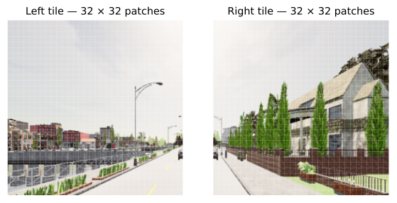
The recorded frame has 1024 columns and 512 rows of pixels. This example removes
the bottom 30%, leaving 358 rows after rounding down. Preprocess.load resizes the cropped image to
896 pixels wide and 448 high using bilinear interpolation, then divides it into two
tiles.
Resizing the 1024-by-358 crop to these dimensions stretches it vertically relative to
its width. Figure 18.3 shows their layout.
Each pixel has red, green and blue components. Preprocessing divides the byte values by 255, subtracts a channel mean and divides by a channel standard deviation. For the red channel, for example, the result is . The corresponding mean and standard deviation are for green and for blue. These constants put the pixels on the scale used by the trained vision encoder.
The resulting array has shape [|2; 448; 448; 3|]: tile, row, column, channel. Vit.forward selects one tile at a
time and calls Vit.tile. That function begins by applying a convolution, using the operation
described in Chap. 11:
  let kernel = Weights.expect w "vit.embeddings.patch_embedding.weight" [| 14; 14; 3; 1024 |] in
  let patches =
    A.conv2d ~padding:Owl_types.VALID image kernel [| 14; 14 |] |> fun x ->
    A.reshape x [| 1024; 1024 |] |> fun x ->
    A.add x (Weights.get w "vit.embeddings.patch_embedding.bias")
  in
  let cls = Weights.get w "vit.embeddings.class_embedding" |> fun x -> A.reshape x [| 1; 1024 |] in
  let pos =
    Weights.get w "vit.embeddings.position_embedding" |> fun x -> A.reshape x [| 1025; 1024 |]
  in
  let x = ref (A.add (Nn.cat [| cls; patches |]) pos) in
The convolution uses a kernel and a stride of 14 in both spatial directions. Each output location therefore corresponds to one non-overlapping patch. The kernel reads three colour channels and produces 1024 features. A tile becomes a grid of 1024-component vectors. Flattening its spatial dimensions gives the array of shape in the code. The two occurrences of 1024 have different meanings: one counts patches, the other counts features per patch.
This is the first use of the word token for an image. An image token is a vector associated with a position in the image sequence. At this point it represents a patch. The vision Transformer will let that vector gather information from the other patches, following the same attention calculation that we have just worked through. Treating patches as a sequence is the central construction of a vision Transformer, or ViT [4].
The code also retrieves a learned class token, cls. It prepends this single row to the
patch rows, then adds a learned positional vector to each row. There are
now 1025 rows. The positional vectors distinguish locations: two patches
with similar colours can begin with different representations because they
occupy different parts of the tile. The class token participates in the encoder’s
computation, and is removed before the patch grid is reduced later in this
section.
18.4.1 Following One Vision Block
The vision encoder repeats a block 24 times. Each block contains an attention calculation and a small network applied separately to every position. Both add their result back to the current array. To understand these additions, first consider the normalization used before each calculation:
let layer_norm w name x =
  let axis = Array.length (A.shape x) - 1 in
  let centered = A.sub x (A.mean ~axis ~keep_dims:true x) in
  (* Explicit population variance: independent of sample-variance conventions. *)
  let variance = A.mean ~axis ~keep_dims:true (A.sqr centered) in
  let normalized = A.div centered (A.sqrt (A.add_scalar variance 1e-6)) in
  A.add (A.mul normalized (Weights.get w (name ^ ".weight"))) (Weights.get w (name ^ ".bias"))
For every row, layer_norm subtracts the row mean and divides by the square
root of its variance plus a small constant. For instance, the row
has mean 2
and variance .
Before the learned scale and bias, its normalized values are approximately
. The keep_dims:true
arguments keep the reduced dimension of size one, allowing Owl to broadcast each
row’s mean and variance over its components. The learned scale and bias then adjust
individual features.
With this helper in place, we can read the body of a vision block. The
loop variable i selects a layer from 0 to 23, and x holds the current sequence:
    let p = Printf.sprintf "vit.encoder.layers.%d" i in
    let qkv = Nn.layer_norm w (p ^ ".norm1") !x |> Nn.linear w (p ^ ".attn.qkv") in
    let attn =
      Nn.attention ~heads:16 ~kv_heads:16 (Nn.cols qkv 0 1024) (Nn.cols qkv 1024 1024)
        (Nn.cols qkv 2048 1024)
      |> Nn.linear w (p ^ ".attn.proj")
    in
    x := A.add !x (A.mul attn (Weights.get w (p ^ ".ls1")));
    let mlp =
      Nn.layer_norm w (p ^ ".norm2") !x
      |> Nn.linear w (p ^ ".mlp.fc1")
      |> Nn.gelu
      |> Nn.linear w (p ^ ".mlp.fc2")
    in
    x := A.add !x (A.mul mlp (Weights.get w (p ^ ".ls2")));
The first linear map packs the query, key and value projections into one array of
width 3072. Three slices recover the groups of 1024 columns. Attention combines
information between positions, and the output projection mixes its heads.
Multiplication by ls1 scales the update feature by feature. Adding that update to !x
creates a residual connection: the block keeps the current representation and adds a
learned change to it.
The next part normalizes the updated rows and passes each through two linear
maps. The first expands the width from 1024 to 4096, the GELU activation changes
the expanded features, and the second returns to 1024. GELU computes
,
where
is the standard normal cumulative distribution function. Our helper evaluates it
through the error function. Another learned scale, ls2, and another residual addition
complete the block.
Attention mixes information between positions; the two linear maps and activation transform the features within each position. Alternating these operations lets a patch representation respond to its surroundings and then transform the gathered information. After 24 blocks, each tile still has 1025 rows of width 1024.
18.4.2 Merging Neighbouring Patches
The language model will receive a shorter sequence than the vision encoder. The implementation drops the class token and combines each group of neighbouring patch vectors into one longer vector. A small grid makes the ordering visible:
let grid = A.init [|4; 4; 1|] float_of_int
let merged =
  A.reshape grid [|4; 2; 2|]
  |> A.transpose ~axis:[|1; 0; 2|]
  |> fun x -> A.reshape x [|2; 2; 4|]
  |> A.transpose ~axis:[|1; 0; 2|]
  |> fun x -> A.reshape x [|4; 4|]
Here the grid has four rows, four columns and one channel. Its entries run from 0 to 15 in row order. The top-left block therefore contains 0 and 1 in its first row, followed by 4 and 5 in its second. The reshape and transpose operations put these four entries into the first output row:
Block 0:  0  1  4  5
Block 1:  2  3  6  7
Block 2:  8  9 12 13
Block 3: 10 11 14 15
A reshape preserves the order of the elements while changing how indices address them. A transpose changes the order of the axes. We need both: consecutive elements initially follow whole image rows, whereas the desired output groups two neighbouring columns from each of two neighbouring rows. The first reshape groups adjacent columns. Transposing moves that group index ahead of the image-row index. The next reshape joins adjacent rows within a group, and the final transpose restores the order of the reduced spatial grid.
The model performs the same operation on its grid, with 1024 channels at each location:
let pixel_shuffle x =
  A.reshape x [| 32; 16; 2048 |] |> A.transpose ~axis:[| 1; 0; 2 |] |> fun x ->
  A.reshape x [| 16; 16; 4096 |] |> A.transpose ~axis:[| 1; 0; 2 |] |> fun x ->
  A.reshape x [| 256; 4096 |]
There are now
positions, each with
features. No learned weights are involved in this rearrangement. The name pixel_shuffle comes
from the original model’s implementation; here the operation reduces the spatial grid
and increases the feature width. The following projection gives the rows the width
expected by the language model:
  Nn.rows !x 1 1024 |> pixel_shuffle |> Nn.layer_norm w "mlp1.0" |> Nn.linear w "mlp1.1" |> Nn.gelu
  |> Nn.linear w "mlp1.3"
It applies layer normalization, a linear map from 4096 to 896, GELU, and a second linear map from 896 to 896. The two tiles are processed with the same weights and their results are concatenated, left tile first. We obtain image features.
Table 18.1 collects the dimensions. It is useful to read it alongside lib/vit.ml:
each row describes a concrete array that the next operation consumes.
18.5 Building the Input Sequence
We now have 512 image rows. The language model needs a sequence that also
contains the question, speed and navigation targets. Simlingo.prompt constructs its text template:
let prompt ~speed ~question =
  if (not (Float.is_finite speed)) || speed < 0. then invalid_arg "invalid speed";
  if String.contains question '<' then invalid_arg "question must not contain special-token syntax";
  "<|im_start|>user\n<img>"
  ^ String.concat "" (List.init 512 (fun _ -> "<IMG_CONTEXT>"))
  ^ "</img>\n"
  ^ Printf.sprintf "Current speed: %.1f m/s. Target waypoint: <TARGET_POINT><TARGET_POINT>. %s"
      speed question
  ^ "<|im_end|><|im_start|>assistant\n"
The markers delimit a user message and the beginning of the assistant’s reply.
Within the user message, <img> and </img> surround 512 copies of <IMG_CONTEXT>. Later in the text, two copies
of <TARGET_POINT> reserve positions for the navigation targets. The speed is formatted as text with
one decimal place. For our scene, that part reads “Current speed: 9.5 m/s.” The
question follows it.
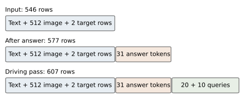
These markers have token IDs of their own. Consequently, the 512 image placeholders occupy exactly 512 positions after tokenization, even though the printed spelling of each marker contains many characters. The complete prompt for the straight-road example contains 546 tokens. Of these, 512 reserve image rows and two reserve target rows; the remaining 32 encode text and message markers.
18.5.1 From Text to Rows
For ordinary text, the tokenizer uses byte-pair encoding, or BPE. It first separates the text into pieces according to rules for letters, numbers, punctuation and spaces. Within a piece, it starts from byte symbols and repeatedly joins adjacent pairs according to a learned merge ranking. Joining stops when no permitted pair remains. A vocabulary lookup then gives the resulting symbols their integer IDs. The vocabulary and merge ranking are part of the saved model assets.
For a small example, ask the supplied tokenizer to encode the first sentence of the answer:
Follow the route.
[12480; 279; 6021; 13]
The four IDs represent Follow, the, route and ., respectively. The leading spaces belong to
the middle two tokens. This explains why decoding concatenates the token bytes
directly: inserting an extra space between every decoded token would change the
sentence. Longer or less familiar words may occupy several tokens. The model’s unit
of generation is the token, so the number of generated steps can differ from the
number of words.
The lookup table has 151655 rows of width 896. Simlingo.embeddings gathers rows from it:
let embeddings w ids =
  A.rows
    (Weights.expect w "qwen.embed_tokens.weight" [| 151655; 896 |])
    (Array.map (fun id -> max 0 (min 151654 id)) ids)
Ordinary vocabulary IDs select their corresponding learned rows. The target placeholder ID, 151662, lies outside this table, so the initial lookup clamps it to an existing row. That temporary row is overwritten by a coordinate embedding during the merge. The image placeholder ID is 151648, and its lookup row is also overwritten. By the time the language model receives the sequence, both kinds of placeholder contain their intended input features.
18.5.2 Replacing the Placeholders
Let us try that replacement with a seven-position sequence and vectors of width three. We use 99 for an image placeholder and 98 for a target placeholder; IDs 0, 1 and 2 are ordinary text. The image and target vectors contain easy-to-recognize numbers:
let ids = [|0; 99; 99; 1; 98; 98; 2|]
let table = A.of_array [|1.; 0.; 0.; 0.; 1.; 0.; 0.; 0.; 1.|] [|3; 3|]
let images = A.of_array [|10.; 11.; 12.; 20.; 21.; 22.|] [|2; 3|]
let points = A.of_array [|30.; 31.; 32.; 40.; 41.; 42.|] [|2; 3|]
let sequence = A.rows table (Array.map (fun id -> min id 2) ids)

let () =
  let image_index = ref 0 and point_index = ref 0 in
  Array.iteri (fun pos id ->
    let replace values index =
      let row = A.get_slice [[!index]; []] values in
      A.set_slice [[pos]; []] sequence row;
      incr index
    in
    if id = 99 then replace images image_index
    else if id = 98 then replace points point_index) ids
id  0:  1  0  0
id 99: 10 11 12
id 99: 20 21 22
id  1:  0  1  0
id 98: 30 31 32
id 98: 40 41 42
id  2:  0  0  1
The sequence length stays seven. Rows at the placeholder positions change, while the text rows retain their lookup values. The two counters track which image or target row to use next. This also gives a reason for the common width: each replacement must fit into one row of the same array.
The model’s merge follows this pattern. Before replacing the target rows, it encodes the coordinates with a small network:
let merge w ids image_features targets =
  if A.shape image_features <> [| 512; 896 |] then invalid_arg "image feature shape";
  if A.shape targets <> [| 2; 2 |] then invalid_arg "two target points required";
  let x = embeddings w ids in
  let points =
    Nn.linear w "wp_encoder.mlp.0" targets
    |> A.relu |> Nn.linear w "wp_encoder.mlp.2" |> A.relu |> Nn.linear w "wp_encoder.mlp.4"
  in
  let image_index = ref 0 and target_index = ref 0 in
  Array.iteri
    (fun pos id ->
      let replace values index = A.set_slice [ [ pos ]; [] ] x (Nn.rows values index 1) in
      if id = 151648 then (
        if !image_index >= 512 then invalid_arg "too many image tokens";
        replace image_features !image_index;
        incr image_index)
      else if id = 151662 then (
        if !target_index >= 2 then invalid_arg "too many target tokens";
        replace points !target_index;
        incr target_index)
      else if id >= 151655 then invalid_arg "unsupported placeholder in prompt")
    ids;
  if !image_index <> 512 || !target_index <> 2 then invalid_arg "prompt placeholder count";
  x
The target encoder maps each two-component point through widths 256, 512 and 896, applying ReLU after the first two linear maps. Both points use the same weights. The network supplies a learned representation of numerical coordinates in the feature space used by the language model. Image rows have reached that width through the vision projection; text rows have reached it through the embedding lookup.
The loop scans the token IDs in order. Each image placeholder
receives the next image row, and each target placeholder receives the
next encoded target. The counts at the end check that the sequence has
consumed all 512 image rows and both target rows. The result, x, has shape
for
our running example.
At this point, the language Transformer receives all three kinds of input through one array interface.
18.6 Generating an Answer
We have reached Qwen2.forward. It accepts the combined array and returns an updated row at
every position. The row at the end of the sequence will supply the next-token scores.
To understand that result, we will follow one language block, using the attention
calculation from Sect. 18.3.
18.6.1 Which Positions Can Read Which?
Text generation proceeds from left to right. A position can use the positions before it and its own input, while later positions are excluded from its attention calculation. We enforce this rule by adding a causal mask to the attention scores. For a sequence of four positions, the mask is
| (18.2) |
Row belongs to query position ; column belongs to key position . Adding zero preserves an allowed score. Adding negative infinity makes its exponential zero in softmax, so the corresponding value receives no weight. The last row can read the whole current sequence, which is what we need when predicting its next token.
The implementation builds this matrix with A.init in the forward function below. For a
flattened element index i, integer division by n gives the row and remainder modulo n
gives the column. Entries whose column exceeds their row receive neg_infinity. This is the same
optional mask accepted by Nn.attention.
18.6.2 Normalizing and Positioning the Features
The language block begins with RMS normalization. It divides each row by the root mean square of its components, then applies a learned scale:
let rms_norm w name x =
  let axis = Array.length (A.shape x) - 1 in
  let variance = A.mean ~axis ~keep_dims:true (A.sqr x) in
  A.mul (A.div x (A.sqrt (A.add_scalar variance 1e-6))) (Weights.get w (name ^ ".weight"))
For the row , the
root mean square is ,
about 3.536. Ignoring the tiny stabilizing constant, normalization gives approximately
before the learned scale. This function scales the row without first subtracting its
mean. The variable variance in the implementation holds the mean square here.
Linear projections of the normalized rows produce queries, keys and values. We must also tell attention where these rows sit in the sequence. The language model does this by rotating pairs of query and key components according to position. For a pair and an angle , the rotated pair is
| (18.3) |
For example, rotating through a quarter turn gives . Different sequence positions produce different rotations, while corresponding query and key components use the same frequency. Their dot product then depends on the difference between their positions. This is rotary position embedding, or RoPE [7].
Here is the implementation used by our model:
let rope_tables n =
  let angles =
    A.init [| n; 32 |] (fun i -> float (i / 32) /. (1e6 ** (float (2 * (i mod 32)) /. 64.)))
  in
  (A.cos angles, A.sin angles)

let rope (cos, sin) x =
  let n = (A.shape x).(0) in
  let heads = (A.shape x).(1) / 64 in
  Array.init heads (fun h ->
      let a = Nn.cols x (h * 64) 32 and b = Nn.cols x ((h * 64) + 32) 32 in
      A.concatenate ~axis:1
        [| A.sub (A.mul a cos) (A.mul b sin); A.add (A.mul b cos) (A.mul a sin) |])
  |> A.concatenate ~axis:1
  |> fun x -> A.reshape x [| n; heads * 64 |]
Each head has 64 components, arranged as 32 pairs. The code pairs
component 0 with 32, component 1 with 33, and so on. Thus the slices a
and b hold the first and second members of all pairs. For sequence position
and pair
, the
angle is .
Early pairs rotate faster with position; later pairs rotate more slowly. rope_tables prepares their
cosines and sines for all positions, and rope applies the two terms of the rotation formula.
Values are passed to attention without this rotation.
18.6.3 Reading a Language Block
The language model has 14 query heads and two key/value heads, each of width 64. Its query projection therefore has width 896, while its key and value projections each have width 128. Seven query heads share one key/value head. This arrangement is called grouped-query attention [8].
We have already seen its implementation in Nn.attention. With heads:14 and kv_heads:2, the integer expression h / (heads / kv_heads)
maps query heads 0–6 to key/value head 0 and query heads 7–13 to key/value head
1. Each query head still computes its own scores and weights. Concatenating its
64-component output with the other heads produces the familiar width of
896.
The remaining part of the block transforms each row through a gated network. One linear map makes a gate, another makes candidate features, and their elementwise product chooses how strongly the candidates contribute. The gate uses the SiLU activation, . Both maps expand the width from 896 to 4864. A final map takes the product back to 896. This combination is commonly called SwiGLU.
We can now read the complete forward function in order:
let forward ?(tap = fun _ _ -> ()) w input =
  let n = (A.shape input).(0) in
  let mask = A.init [| n; n |] (fun i -> if i mod n > i / n then neg_infinity else 0.) in
  let tables = rope_tables n in
  let x = ref input in
  for i = 0 to 23 do
    let p = Printf.sprintf "qwen.layers.%d" i in
    let z = Nn.rms_norm w (p ^ ".input_layernorm") !x in
    let q = Nn.linear w (p ^ ".self_attn.q_proj") z |> rope tables in
    let k = Nn.linear w (p ^ ".self_attn.k_proj") z |> rope tables in
    let v = Nn.linear w (p ^ ".self_attn.v_proj") z in
    let attn =
      Nn.attention ~mask ~heads:14 ~kv_heads:2 q k v |> Nn.linear w (p ^ ".self_attn.o_proj")
    in
    x := A.add !x attn;
    let z = Nn.rms_norm w (p ^ ".post_attention_layernorm") !x in
    let gate = Nn.linear w (p ^ ".mlp.gate_proj") z |> Nn.silu in
    let up = Nn.linear w (p ^ ".mlp.up_proj") z in
    x := A.add !x (Nn.linear w (p ^ ".mlp.down_proj") (A.mul gate up));
    if i = 0 then tap "qwen_layer1" !x
  done;
  Nn.rms_norm w "qwen.norm" !x
The first residual addition combines the input with the attention update. The second combines that result with the gated-network update. Repeating the block changes the representation at each position while preserving the array shape. After all 24 blocks, a final RMS normalization prepares the rows for the output heads.
The optional tap function records intermediate arrays when we ask the executable for
a diagnostic dump. Its default does nothing. It gives us a convenient way to
inspect the first block without changing the numerical path through the
model.
Let us follow the last row through this function once. Its query can attend to all positions in the current sequence: image features, navigation targets, prompt text and any answer tokens already appended. The resulting row has 896 components. The next function maps those components to one score per vocabulary entry:
let logits w hidden = Nn.rows hidden ((A.shape hidden).(0) - 1) 1 |> Nn.linear w "qwen.lm_head"
These scores are called logits. The output has shape . Our generation rule selects the largest score. Softmax would preserve their ordering, so selecting the largest logit gives the same token as selecting the largest softmax probability.
18.6.4 Appending One Token at a Time
The first call predicts ID 12480, which decodes to Follow. We append that token’s
embedding to the input sequence. The next call sees one more row and predicts the
following token. The recursive loop carries out this process:
let generate ?(tap = fun _ _ -> ()) ~max_new_tokens w input =
  if max_new_tokens < 1 || max_new_tokens > 100 then invalid_arg "max-new-tokens must be 1..100";
  let rec loop step input ids =
    if step = max_new_tokens then (Array.of_list (List.rev ids), input)
    else (
      Printf.eprintf "language token %d/%d (sequence %d)\n%!" (step + 1) max_new_tokens
        (A.shape input).(0);
      let hidden = Qwen2.forward ~tap:(if step = 0 then tap else fun _ _ -> ()) w input in
      let logits = Qwen2.logits w hidden in
      if step = 0 then tap "first_logits" logits;
      let id = Nn.argmax logits in
      let input = Nn.cat [| input; embeddings w [| id |] |] in
      if id = 151645 then (Array.of_list (List.rev (id :: ids)), input)
      else loop (step + 1) input (id :: ids))
  in
  let ids, input = loop 0 input [] in
  Printf.eprintf "driving head\n%!";
  let route, speed = driving w input in
  (ids, route, speed)
The argument input is the growing embedding sequence. The list ids holds the generated
IDs in reverse order, so adding another ID takes constant time. Before returning, the
function reverses the list and converts it to an array. step counts how many tokens have
been generated.
At each step, the function computes updated hidden rows, obtains the last row’s logits, finds the largest one and appends the selected token’s embedding. The stopping token has ID 151645. Its embedding is appended before the function leaves the loop, so it is present in the context used by the driving pass. The tokenizer decodes the accumulated ordinary token bytes into the displayed answer and omits this special end marker.
The training examples for this question append the text Waypoints: to the commentary,
which explains the ending in our generated answers. In this example, EOS follows
that text, and the program then appends the driving queries.
This rule is greedy decoding: choose the highest-scoring next token at every step.
The loop above recomputes the Transformer over the whole current sequence on each
call. The parameter max_new_tokens supplies a second stopping condition; its default and largest
allowed value are both 100. The JSON field eos_reached tells us whether the answer reached its
end marker.
For the straight-road scene, the 546 input rows grow to 577 after 31 generated tokens, including that marker. Figure 18.4 shows the sequence before and after generation. The driving queries will extend it once more. Before adding them, let us look at the work repeated during generation.
18.6.5 Reusing Keys and Values
After predicting Follow, our loop processes 547 rows to predict the next token.
Only one embedding is new. The other 546 rows have already passed through all 24
language blocks. We can save much of that repeated work.
Recall the causal mask: an earlier position cannot read a later one. Appending a token therefore leaves the earlier positions’ representations unchanged. Their keys and values are unchanged too, at every layer. A key/value cache, usually shortened to KV cache, keeps these arrays for the next call. The new query still reads the whole available prefix, but we only compute projections and block updates for the new row.
Figure 18.5 shows this with four positions. In the upper panel, all four query rows take part in attention. In the lower panel, only is new. It reads the three saved keys and the new key, then combines the corresponding four values. Its output matches the last row of the full calculation. The keys and values carry information forward; the attention weights for the new query are calculated afresh.
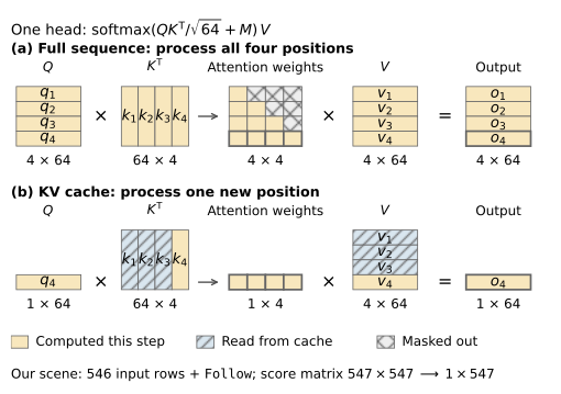
The first pass still processes all 546 input rows. This pass, often called
prefill, fills the caches and predicts Follow. The next call takes just that
token’s embedding. Each layer projects this row into queries, keys and values,
appends its keys and values to the cache, and reads the 547 positions now
available. For each attention head, the score array has one row and 547
columns.
The module Qwen2_cached allocates the storage when a request begins:
let create ~capacity weights =
  if capacity < 1 then invalid_arg "KV cache capacity must be positive";
  let layers =
    Array.init 24 (fun _ ->
        { keys = A.empty [| capacity; 128 |]; values = A.empty [| capacity; 128 |] })
  in
  { weights; layers; capacity; length = 0 }
Each of the 24 layers owns a pair of arrays. Their width is 128: two key/value
heads with 64 components each. The capacity covers the input, the allowed answer
length and the 30 driving queries. The field length counts the positions already
processed. Keeping a length separately lets us append rows without allocating a
larger cache at every step.
Within layer i, the projections produce q, k and v for the new rows. Here past is
the cached length, n is the number of new rows and total = past + n. The
following lines store the new keys and values and pass the occupied prefix to
attention:
    let layer = cache.layers.(i) in
    A.set_slice [ [ past; total - 1 ]; [] ] layer.keys k;
    A.set_slice [ [ past; total - 1 ]; [] ] layer.values v;
    let keys = Nn.rows layer.keys 0 total and values = Nn.rows layer.values 0 total in
    let attn = Nn.attention ?mask ~heads:14 ~kv_heads:2 q keys values
               |> Nn.linear w (p ^ ".self_attn.o_proj") in
For the call that processes Follow, past is 546 and n is 1. The slice writes row
546, using zero-based indices. All 547 stored positions are visible to this row, so mask
is None. The same position number determines the RoPE rotation for its query and
key; numbering starts at past on each call. The keys already stored in the cache keep
their rotations. After all layers have processed the new rows, the cache length
becomes total.
On an Intel Core i9-13900KF with four BLAS threads, KV caching gave the straight-road run a speedup over the full-sequence implementation. Across the four recorded scenes, speedups ranged from to . These measurements cover the complete inference process, from loading the weights to producing the waypoints. Both versions generated identical token sequences, with only small floating-point differences in the waypoint coordinates. The completed prefix can also be reused when we add the driving queries.
18.7 Predicting Waypoints
The model has now produced a sentence. To obtain coordinates, it appends two groups of learned rows: 20 route queries and ten speed queries. Each query has 896 components, so it fits the same sequence as the input and answer embeddings. These rows are saved model parameters. Their order assigns an output position to each query.
A driving query is distinct from the projected query in an attention head. The driving query is a row appended to the sequence; the language blocks will project it into attention queries, keys and values in the usual way. Because it appears after the answer, it can gather information from the earlier input and answer positions. The causal ordering also lets later driving queries use earlier query positions. The route queries come first, followed by the speed queries.
Here is the complete driving function:
let driving w input =
  let route_queries =
    Weights.expect w "driving.query_embeds_wps" [| 1; 20; 896 |] |> fun x ->
    A.reshape x [| 20; 896 |]
  in
  let speed_queries =
    Weights.expect w "driving.query_embeds_speed" [| 1; 10; 896 |] |> fun x ->
    A.reshape x [| 10; 896 |]
  in
  let hidden = Qwen2.forward w (Nn.cat [| input; route_queries; speed_queries |]) in
  let start = (A.shape hidden).(0) - 30 in
  let route =
    Nn.rows hidden start 20
    |> Nn.linear w "driving.route_head.0"
    |> Nn.silu
    |> Nn.linear w "driving.route_head.2"
    |> Nn.silu
    |> Nn.linear w "driving.route_head.4"
    |> A.cumsum ~axis:0
  in
  let speed =
    Nn.rows hidden (start + 20) 10
    |> Nn.linear w "driving.speed_wps_head.0"
    |> Nn.silu
    |> Nn.linear w "driving.speed_wps_head.2"
    |> A.cumsum ~axis:0
  in
  (route, speed)
For our example, the call to Qwen2.forward receives
rows.
The variable start identifies the first of its final 30 rows. The route head takes 20 rows
from there; the speed head takes the remaining ten. Both heads act on the final
normalized language-model states.
The cached path reaches the same 607-position context by appending a smaller
chunk. When EOS is selected, 576 positions have already been processed; EOS
itself has yet to enter the cache. The function Simlingo_cached.generate
therefore passes EOS and the 30 driving queries together as 31 new rows. They
read the cached prefix, while a causal mask preserves their order within the
chunk.
The route head changes each row’s width from 896 to 512, then to 256, then to two. The speed head uses widths 896, 256 and two. Their intermediate layers apply SiLU. The two output components represent a displacement in the forward and right directions. Each head has its own learned weights, allowing the two groups to express their different sampling conventions.
18.7.1 From Displacements to Positions
The last operation in both branches is A.cumsum ~axis:0. It adds successive displacements along the
point sequence. We can see its effect with three small steps:
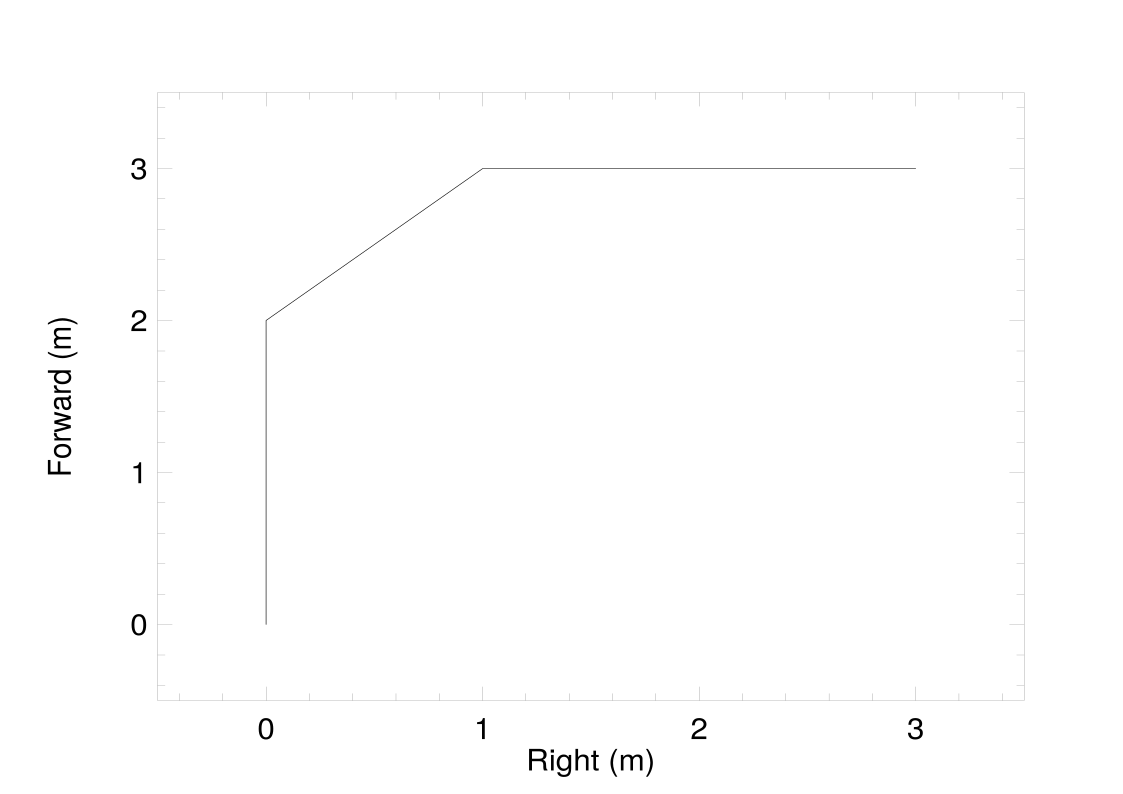
let displacements = A.of_array [|2.; 0.; 1.; 1.; 0.; 2.|] [|3; 2|]
let waypoints = A.cumsum ~axis:0 displacements
Point 1: (2.0, 0.0)
Point 2: (3.0, 1.0)
Point 3: (3.0, 3.0)
The first step takes us from to . The second adds and takes us to . The third adds and takes us to . Figure 18.6 plots these steps. In symbols, if the head produces displacements , the returned point at index is
| (18.4) |
The sum operates along rows, keeping the two coordinate columns separate. Summing along the feature axis would combine forward and right components within each point, which would have a different meaning.
The final arrays both contain positions measured from the same ego origin. To recover a displacement between successive points, subtract them. For a speed-waypoint sequence, divide the length of such a displacement by 0.25 seconds to obtain the average speed over that interval. Use the origin as the point before the first prediction. In our straight-road example, the first speed waypoint is approximately metres. Its distance from the origin is metres, giving an average speed of metres per second over the first interval, close to the input speed of 9.5 metres per second.
For the route sequence, the training targets are sampled by distance along the path. Their approximately one-metre spacing describes geometry. The speed waypoints are sampled by time, so wider spacing means more distance covered during the same interval. This is why a fast-moving scene can have speed waypoints extending beyond the end of the 20-point route.
The numerical connection between language and action is now visible in the code. The answer embeddings remain in the sequence when the driving queries are evaluated. Attention makes them available to those queries together with the image and navigation information. The coordinate heads read the resulting continuous vectors and produce floating-point coordinates. We have followed the path from a sentence in the context to the arrays used to describe motion.
18.8 Running the Model
The four short programs live in the examples/ subdirectory of
code/chap18_autonomous_driving/. Each prints the values used in its explanation;
the waypoint example also writes its plot. They are useful places to experiment
before loading the model. Change a value vector in the attention example, or put two
distinctive numbers next to each other in the patch grid, and follow where they
appear in the result.
18.8.1 Loading the Trained Arrays
The full model lives in simlingo-owl/. It needs Owl, Yojson for JSON files,
Sha for checksums, and Dune to build the modules. From that directory:
opam install owl yojson sha dune
dune build
The repository also includes Dockerfile.book, a local extension of the book
image that adds Yojson and Sha. It is the environment used to execute the full
examples printed here.
The model weights come from the SimLingo project’s trained checkpoint [10].
This chapter uses the epoch=013.ckpt/pytorch_model.pt checkpoint and the
tokenizer assets of OpenGVLab/InternVL2-1B. The converter’s --base argument names a
local directory containing that model’s configuration and tokenizer files. The model
project’s download instructions provide the checkpoint; the companion README
records the expected layout.
Conversion is a one-time preparation step. It reads the checkpoint,
combines its low-rank updates with the corresponding weight matrices,
and writes single-precision NumPy arrays. A low-rank update stores
a change as the product of two smaller matrices. For this checkpoint, the
converter scales that product by two and adds it to the base matrix:
. The
result is the single weight used during inference. The converter also transposes
matrices into the layout used by Nn.linear and changes convolution kernels into Owl’s spatial,
input-channel, output-channel order.
The converter uses Python with NumPy and PyTorch to read the checkpoint. Set CHECKPOINT
and BASE to those local paths and run:
python tools/convert.py --checkpoint "$CHECKPOINT" \
  --base "$BASE" --out artifacts/weights
The destination contains 653 weight arrays, totalling about 3.76 GB, plus a manifest and tokenizer files. We recommend 16 GB of system RAM for this workflow. In a complete run of the straight-road example, peak resident memory was 4.41 GB; the separate weight-conversion process used 3.06 GB at its peak.
Weights.get loads an array on first use, verifies its checksum and shape, and retains it for
later calls. Subsequent generated tokens reuse the loaded weights. The names passed
to Nn.linear, such as qwen.layers.0.self_attn.q_proj, locate the appropriate arrays in that collection.
18.8.2 Replaying the Straight-Road Frame
The demo/straight/ directory contains the frame and the numerical inputs used
throughout the chapter. A small wrapper reads its input record, converts the PNG
into an RGB PPM file and invokes the OCaml executable. It needs Pillow to decode
the PNG. From simlingo-owl/, run:
python tools/run_frame.py --frame demo/straight \
  --weights artifacts/weights --out artifacts/replay-straight
To use the cache described in Sect. 18.6.5, add --kv-cache and choose a new
output directory:
python tools/run_frame.py --frame demo/straight \
  --weights artifacts/weights --kv-cache \
  --out artifacts/replay-straight-cached
The wrapper prints progress and saves output.json and run.log in the output
directory. The full-sequence version takes a few minutes on CPU. During generation,
its progress lines give the token step and sequence length; the cached version reports
the cached length and the number of new rows. The final JSON contains
the answer, generated token IDs, the end-marker flag and both waypoint
arrays.
The executable can also be called directly. Once the wrapper has prepared the PPM file, the equivalent command is:
OPENBLAS_NUM_THREADS=4 OMP_NUM_THREADS=4 \
  _build/default/bin/main.exe \
  --weights artifacts/weights \
  --image artifacts/replay-straight/frame.ppm \
  --speed 9.5 --targets demo/straight/targets.json \
  --crop-bottom 0.3 \
  --question 'What should the ego do next?' \
  --output artifacts/replay-straight/direct.json
The recorded target file preserves the navigation coordinates shown in rounded
form at the start of the chapter. The crop argument preserves the image preparation
used by that example. To inspect the internal arrays, create a directory and supply it
through --dump; the executable saves the pixel array, projected image features,
merged input embeddings, first-layer states and first-step logits as NumPy
files.
18.8.3 Reading the Other Scenes
Figure 18.7 places the straight-road example beside a bend and a closer following scene. All three use the question from the opening. In each coordinate plot, circles show route points and crosses show speed waypoints. The horizontal axis measures rightward displacement, while the vertical axis measures forward displacement.
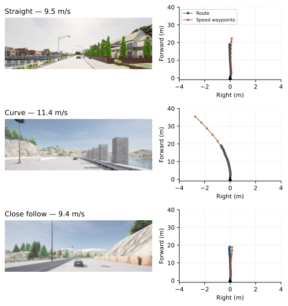
In the straight-road scene, both sequences stay near the forward axis. The speed waypoints extend farther than the route, reflecting their time-based horizon. In the bend, the target points have negative lateral coordinates and both predicted sequences bend left. Its answer is:
Follow the route. Accelerate to drive with the target speed.
Waypoints:
In the close-following scene, the input speed is 9.4 metres per second. The model says:
Follow the route. Decelerate to stay behind the maroon car
that is to the front. Waypoints:
The first three speed-waypoint displacements have lengths of about 1.99, 1.61 and 1.85 metres. At the input speed, travelling for 0.25 seconds would cover 2.35 metres. These predicted intervals therefore describe slower movement. The first three distances decrease and then increase.
The earlier demo/brake/ frame from the same recording produces an
instruction to accelerate even though the lead car is stopped. In the later
demo/close_follow/ frame, the model recommends decelerating. Each input
contains one image, the ego speed and navigation targets; the lead car’s velocity is
not supplied.
To run another retained scene, change the wrapper’s --frame argument and give it a new
output directory. Start by comparing its input.json with the straight-road input.
Then examine the answer, the first speed-waypoint displacement and the shape of the
route. These are three readable entry points into the same computation we have
followed through the source.
18.9 Summary
We began with a camera frame, a speed, two navigation targets and a question. The vision encoder turned image patches into vectors; the tokenizer and embedding table did the same for text; a small network encoded the target coordinates. Placeholder replacement assembled these rows into one sequence.
Attention let positions gather information from that sequence. The vision and language blocks combined attention with normalization, residual additions and per-position networks. The generation loop used the final language row to choose a token, appended its embedding and repeated until the answer ended. Keeping each layer’s keys and values let later steps reuse the prefix. Finally, learned driving queries gathered information from the completed context, and two output heads produced displacements whose cumulative sums gave the waypoints.
These operations give us a way to approach another VLA implementation. Begin with its inputs and outputs. Follow how each input becomes an array, identify where the arrays meet, and trace how the resulting states become words or coordinates. With the shapes beside us and a few small examples to check the transformations, we can read a large model as a sequence of familiar OCaml computations.
Bibliography
- [1]
- Dosovitskiy, A., Ros, G., Codevilla, F., López, A., Koltun, V.:
CARLA: An Open Urban Driving Simulator. In: CoRL (2017).
https://arxiv.org/abs/1711.03938 - [2]
- Renz, K., Chen, L., Arani, E., Sinavski, O.: SimLingo: Vision-Only
Closed-Loop Autonomous Driving with Language-Action Alignment. In:
CVPR (2025).
https://arxiv.org/abs/2503.09594 - [3]
- Vaswani, A., et al.:
Attention Is All You Need. In: Advances in Neural Information Processing
Systems (2017).
https://arxiv.org/abs/1706.03762 - [4]
- Dosovitskiy, A., et al.: An Image is Worth 16x16 Words: Transformers for
Image Recognition at Scale. In: ICLR (2021).
https://arxiv.org/abs/2010.11929 - [5]
- Yang, A., et al.: Qwen2 Technical Report (2024).
https://arxiv.org/abs/2407.10671 - [6]
- OpenGVLab: InternVL2-1B model configuration and tokenizer.
https://huggingface.co/OpenGVLab/InternVL2-1B. Accessed 16 November 2026 - [7]
- Su, J., et al.: RoFormer:
Enhanced Transformer with Rotary Position Embedding. Neurocomputing
568, 127063 (2024).
https://arxiv.org/abs/2104.09864 - [8]
- Ainslie, J., et al.: GQA:
Training Generalized Multi-Query Transformer Models from Multi-Head
Checkpoints. In: EMNLP (2023).
https://arxiv.org/abs/2305.13245 - [9]
- Lages, J.: Transformers KV Caching Explained. Medium (2023).
https://medium.com/@joaolages/kv-caching-explained-276520203249. Accessed 16 November 2026 - [10]
- Renz, K., et al.: SimLingo source and trained models.
https://github.com/RenzKa/simlingo. Accessed 16 November 2026