CHAPTER 05
N-Dimensional Arrays
The -dimensional
array is the fundamental building block in numerical computing libraries,
e.g., NumPy and SciPy. It is the core dense data structure and many advanced
numerical functions are built on top of it, including linear algebra, optimisation, and
algorithmic differentiation. In fact, the rest of this book is built upon it. In this chapter,
we introduce the Ndarray module and its core functions. We then pay particular
attention to its two key and frequently used functionalities: slicing and broadcasting.
Finally, we briefly explain the concept of a tensor, similar to but different from the
-dimensional
array.
5.1 Ndarray
An -dimensional
array (a.k.a. ndarray) is the most fundamental data type in a numerical library for
building scientific computing applications. Scalar-based computations are easy to
understand but can become cumbersome when working with large arrays. Ndarray is
the key data structure in many mainstream numerical libraries and software,
including NumPy, Julia, and TensorFlow. This chapter introduces Owl’s Ndarray, a
fundamental module in OCaml numerical computing, and the basic functionalities it
provides.
5.1.1 Types
We begin by looking at the data types used in Ndarray, which is built directly on
top of OCaml’s native Bigarray data structure. The Bigarray module is used to
express large, multi-dimensional numerical arrays, and is designed to enable
efficient sharing of large numerical arrays between OCaml code and C or
FORTRAN numerical libraries. More specifically, Ndarray is defined based on the
Bigarray.Genarray submodule:
type ('a, 'b) t = ('a, 'b, Bigarray.c_layout) Bigarray.Genarray.t
The type parameters of Genarray.t specify the OCaml element type, storage
kind, and memory layout of a multi-dimensional array. Based on different
combinations of (’a, ’b), Ndarray supports four combinations of number type and
precision: single precision float (S), double precision float (D), single precision
complex number (C), and double precision complex number (Z). These are all
accessed by modules Ndarray.S, Ndarray.D, etc. In what follows, unless otherwise
stated, we will use the double precision Ndarray.D module which is aliased to the
Arr module.
The Ndarray module is designed to use row-major layout (c_layout) in its
implementation. This indicates that adjacent elements along the last dimension are
contiguous in memory, compared to FORTRAN layout where this holds along the
first dimension. From the perspective of designing Owl, our reasons for making this
decision are as follows.
- Mixing memory layouts causes bugs. In particular, indexing in FORTRAN
starts from 1 while indexing in C starts from 0, and many native OCaml
data structures such as
ArrayandListall index from 0. So sticking with C-layout avoids many clashes when using Owl. - Supporting both layouts adds considerable complexity when implementing the underlying functions. Code which performs well on one layout may not do well on the other, and so many functions would require different implementations for different layouts. This would add much complexity and significantly increase the code base for only marginal benefits.
Ndarrayhas rather different design principles compared toBigarray. The latter serves as a basic tool for operating on a chunk of memory living outside the OCaml heap, and facilitates exchanging data between different libraries (including FORTRAN ones). The numerical library we use here focuses on providing high-level numerical functions allowing programmers to write concise analytical code. The simple design and small code base outweigh the benefits of supporting both layouts.
Note that in Owl, a matrix is just a special case of an
-dimensional
array, and you can add a matrix and a 2-dimensional ndarray of compatible shape
and element kind. In fact many functions in the Matrix module simply call the same
functions in Ndarray.
5.1.2 Ndarray Creation and Properties
We start by introducing several groups of key functions provided by Ndarray. The
first group is the creation functions that generate dense data structures. The most
frequently used are probably empty, create, zeros, and ones. These functions
return ndarrays of the specified shape.
Note that the empty function allocates storage without initialising its elements.
This avoids the cost of filling the array, but its contents must be set before use. The
other three are hopefully self-explanatory: zeros and ones fill the allocated memory
with zeros and ones respectively, whereas the create function fills the memory with
the specified value.
If you need random numbers, you can use another three creation functions that
return ndarrays in which the elements follow specified distributions: uniform,
gaussian, and bernoulli. You can provide optional distribution parameters,
e.g.,
and
for a Gaussian distribution; their defaults are 0 and 1 respectively.
We sometimes need to generate numbers equally spaced between bounds, for
example when generating intervals or plotting figures. The sequential and
linspace functions serve that purpose, producing ndarrays filled with evenly spaced
numbers. The former takes a shape and optional starting value and step,
which need not be an integer; the latter takes endpoints and a number of
points.
If these do not satisfy your requirements, Ndarray provides more flexible means
that give you more control over initialisation via the init and init_nd functions.
The first only passes 1-dimensional indices to a user-defined function, while the
second passes n-dimensional indices and incurs the extra cost of computing
them. The example below creates an ndarray where all the elements are even
numbers:
# let x = Arr.init [|6;8|] (fun i -> 2. *. (float_of_int i));;
val x : Owl.Arr.arr =

   C0 C1 C2 C3 C4 C5 C6 C7
R0  0  2  4  6  8 10 12 14
R1 16 18 20 22 24 26 28 30
R2 32 34 36 38 40 42 44 46
R3 48 50 52 54 56 58 60 62
R4 64 66 68 70 72 74 76 78
R5 80 82 84 86 88 90 92 94
After creation, there are various functions that obtain the properties of the
ndarray. For example, given ndarrays x and y, the following functions are commonly
used:
shape xreturns the shape ofxnum_dims xreturns the number of dimensions ofxnth_dim x nreturns the size of the -th dimension ofxnumel xreturns the number of elements inxnnz xreturns the number of non-zero elements inxdensity xreturns the fraction of non-zero elements inxsize_in_bytes xreturns the size of the element storage ofxin bytessame_shape x ychecks whetherxandyhave the same shapekind xreturns the element kind of ndarrayx
5.1.3 Map, Fold, and Scan
Three typical generic operations are worth special attention: map, fold, and scan.
The map function transforms one ndarray to another by applying the provided
function to every element in the original ndarray. For example, the code below:
let y = Arr.map (fun a -> a +. 1.) x;;
adds
1 to every element in the ndarray x, then returns a new ndarray y. The
map function in Ndarray returns a fresh array without modifying the input,
provided the supplied function does not itself mutate it. If your transformation
function needs the index of the element being operated on, the mapi function
passes its flattened, zero-based index; mapi_nd passes an array of coordinates
instead.
The fold function is sometimes referred to as “reduction” in other languages. It
has a named parameter called axis that specifies the axis along which you want to
fold the given ndarray. The axis parameter is optional. If you do not specify one, the
ndarray will be folded along all the dimensions into a single element (that is, a
one-dimensional ndarray of length one). The fold function folds from the left, and
requires an initial value for the folding. The code below demonstrates how to
implement your own sum function. It adds the elements along the selected axis
and returns an ndarray by folding the function +. with an initial value of
0.
let sum ?axis x = Arr.fold ?axis ( +. ) 0. x;;
The functions sum, sum’, prod, prod’, min, min’, mean, and mean’ all perform
reductions with various functions. The prime ending indicates that the function
returns a number rather than an ndarray. As with map, if indices are required, the
foldi function passes in 1-dimensional indices.
Finally, scan is analogous to a combination of map and fold, accumulating values
along the specified axis but not changing the shape of the input. For example,
consider generating a cumulative distribution function from a discrete probability
mass function, as introduced in Chap. 3. Several functions belong to this group, such
as cumsum, cumprod, cummin, cummax. Again, the scani function accepts cumulative
functions that need index information.
Many common operations on ndarrays can be decomposed as a series of map,
fold, and scan operations. The map and reduce operations also inspire
the MapReduce programming model [4]. The Ndarray module includes a
comprehensive set of vectorised element-wise mathematical functions. This
means you can apply them directly on an ndarray and the function will be
automatically applied to every element in the ndarray. For binary math operators,
there are add, sub, mul, etc. For unary operators, there are sin, cos, abs,
etc.
Conceptually, all of these can be implemented using just map, fold, and scan. For
example, to make your own vectorised sin function, you need only execute
Arr.map sin x. However, this may well be slower than the native vectorised
functions, which are implemented in C code for efficiency.
5.1.4 Comparison Functions
The comparison functions in Ndarray can be divided into several groups.
The first group compares two ndarrays and returns a boolean value, such as
equal, less, and greater. The second compares two ndarrays element by element
and returns a 0-1 ndarray of the broadcast result shape, with 1 where the predicate is
satisfied and 0 otherwise: elt_equal, elt_not_equal, etc. The third is similar to the
first, but compares an ndarray with a scalar value, and returns a boolean:
equal_scalar, not_equal_scalar, etc. The fourth is similar to the second but
compares an ndarray with a scalar, and returns a 0-1 ndarray: elt_equal_scalar,
elt_less_scalar, etc.
We generally recommend using the appropriate operators rather than calling these functions directly as it leads to more concise code.
For example, the following code shows two ways to retain all elements greater than 0.5 and set the rest to 0 in an ndarray of finite values.
let y = Arr.map (fun a -> if a > 0.5 then a else 0.) x;;
let z = Arr.((x >.$ 0.5) * x);;
The operator version leads to more concise code and can be faster because the loops run in C rather than OCaml, at the price of an additional temporary mask. The actual performance depends on the input size and environment. Please refer to the Appendix A to learn about all these operators.
5.1.5 Iteration Functions
As with native OCaml arrays, you can use iter and iteri to iterate over all the
elements in an ndarray. One common use case is to check if one or more predicates
are satisfied and there is a special set of iteration functions to help you in this task:
is_zero, is_positive, is_negative, is_nonpositive, is_nonnegative,
and is_normal, etc. All take an ndarray as input and return a boolean
value.
More complex predicates can be tested using the three functions exists,
not_exists, and for_all while passing in arbitrarily complicated functions that
return a boolean. While these functions only tell us whether the predicates are met
or not, the filter function can return the 1-dimensional indices of those elements
that satisfy the predicates.
Processing flattened 1-dimensional indices avoids the cost of converting them to
n-dimensional indices. However, if you do need n-dimensional indices, you can use the
functions ind and i1d to convert between flattened and n-dimensional indices. Both
are defined in the Owl.Utils module. Note that you need to pass in the
original ndarray because the shape information is required for calculating index
conversion.
5.1.6 Manipulation Functions
In addition to those we have introduced, the Ndarray module contains
many useful functions to manipulate ndarrays. For example, you can tile
and repeat an ndarray along a specified axis. Let’s first create a sequential
ndarray.
# let x = Arr.sequential [|3;4|];;
val x : Owl.Arr.arr =

   C0 C1 C2 C3
R0  0  1  2  3
R1  4  5  6  7
R2  8  9 10 11
The code below tiles x twice along each dimension.
# let y = Arr.tile x [|2;2|];;
val y : Owl.Arr.arr =

   C0 C1 C2 C3 C4 C5 C6 C7
R0  0  1  2  3  0  1  2  3
R1  4  5  6  7  4  5  6  7
R2  8  9 10 11  8  9 10 11
R3  0  1  2  3  0  1  2  3
R4  4  5  6  7  4  5  6  7
R5  8  9 10 11  8  9 10 11
The repeat function replicates each element in its adjacent cell along the
specified dimension, as shown below.
# let z = Arr.repeat x [|2;1|];;
val z : Owl.Arr.arr =

   C0 C1 C2 C3
R0  0  1  2  3
R1  0  1  2  3
R2  4  5  6  7
R3  4  5  6  7
R4  8  9 10 11
R5  8  9 10 11
You can also expand the dimensionality of an ndarray, or squeeze out dimensions
having only one element, or pad elements around an existing ndarray, using the
functions expand, squeeze, and pad.
Another two useful functions are concatenate and split. The concatenate
function allows concatenation of an array of ndarrays along the specified axis, given
that the dimensions other than that on which they are concatenated are equal. There
are two operators associated with concatenation for matrices: @|| concatenates
horizontally (i.e. along axis 1); and @= for concatenating vertically (i.e. along axis
0). split is then the inverse operation of concatenation. You can also sort
an ndarray with sort, which returns a sorted copy; sort_ modifies it in
place.
Another feature we will use frequently in this book is to convert between ndarrays
and normal arrays using conversion functions of_array and to_array.
5.1.7 Serialisation
In data analysis tasks we often need to save temporary results and later reload
them. This process requires the serialisation and de-serialisation functions save and
load.
With the help of the tool
npy-ocaml1,
we can save and load files in the NPY binary file format from NumPy. It stores all of
the shape and data type information necessary to reconstruct the array correctly,
even on another machine with a different architecture. It is a widely used serialisation
format in numerical tasks. The corresponding functions are save_npy and load_npy;
the stored element kind must match the module used to load the array. By using
these functions, we can easily interact with the Python-world data from
OCaml.
5.2 Slicing
Slicing in ndarray is the operation that extracts part of an ndarray or a matrix according to a slice definition, an index list that indicates which indices should be accessed and in what order for each dimension of the value being sliced. Indexing and slicing are arguably the most important ndarray functions in any numerical library. Owl’s flexible design significantly simplifies the code, allowing us to write concise algorithms. In this section we will introduce ndarray basic and fancy slicing, which differ in how the slice is defined.
5.2.1 Slice Definition
In basic slicing, each dimension in the slice definition is specified by a list of up to
three integers, [start;stop;step]. Ndarray provides two functions get_slice
and set_slice to retrieve and assign slice values respectively. Both accept
an int list list as the slice definition, where every list element in the
int list list is assumed to be a range. For example, [ []; [2]; [-1;3] ] is
equivalent to the full slice definition [ R []; R [2]; R [-1;3] ] in fancy slicing
notation shown below.
type index =
  Owl_types_common.index =
    I of int
  | L of int list
  | R of int list
The fancy slicing is defined by an index list that uses three type constructors.
I simply specifies a numeric index, so [ I 2; I 5 ] returns a 1 x 1 matrix
containing the element at position (2, 5). L specifies a list of indices, so
[ I 2; L [5;3] ] returns a 1 x 2 matrix with the elements at (2, 5) and (2, 3)
in the original matrix. Finally, R specifies a range of indices. Similarly to get_slice,
the get_fancy s x retrieves a slice of x defined by s, whereas set_fancy s x y
assigns the slice of x defined by s according to values in y. Note that y must have
the same shape as that defined by s. For example, these two slices of x are
equivalent:
let x = Arr.sequential [|10; 10; 10|];;
Arr.get_slice [ []; [0;8]; [3;9;2] ] x;;
Arr.get_fancy [ R[]; R[0;8]; R[3;9;2] ] x;;
Note that both get_slice and get_fancy return a copy. NumPy basic slicing
returns a view, whereas its advanced indexing returns a copy. In Owl, set_slice and
set_fancy modify the original data in place.
The operators for indexing and slicing are built on the extended indexing operators introduced in OCaml 4.06. In the slicing system, they are used as aliases for the slicing functions we introduced above:
.%{get.%{-:set.${get_slice.${-:set_slice.!{get_fancy.!{-:set_fancy
For example, we can use .%{ } for indexing as follows:
open Arr;;
let x = sequential [|10; 10; 10|] in
let a = x.%{2; 3; 4} in
x.%{2; 3; 4} <- 111.;;
Another example uses the .!{ } operator for fancy slicing:
open Arr;;
let x = sequential [|10; 10; 10|] in
let a = x.!{L [2;2;1]; R [6;-1]; I 5} in
let b = zeros (shape a) in
x.!{L [2;2;1]; R [6;-1]; I 5} <- b;;
5.2.2 Conventions and Examples
These definitions of slicing may look complicated. The following rules can help write correct slice definitions. These conventions can be equally applied to both basic and fancy slicing. They resemble those in NumPy, but Owl includes the stop index when reached by the step, infers a descending step when needed, and retains singleton dimensions. If you already know how to slice n-dimensional arrays in NumPy, you should find them easy to follow.
- Rule #1: The format of the range
definition follows
R [ start; stop; step ].startspecifies the starting index,stopspecifies the inclusive stopping bound, andstepspecifies the step size. You do not have to specify all three variables in the definition; see the following rules. - Rule #2: All three variables
start,stop, andstepcan take both positive and negative values, butstepis not allowed to be zero. Positive step indicates that indices will be visited in increasing order fromstarttostop; and vice versa. - Rule #3: For
startandstopvariables, non-negative values refer to a specific index while a negative value “a” will be translated inton + awherenis the size of that dimension. E.g.,[ -1; 0 ]indicates the slice from the last index to the first. - Rule #4: If you pass in an empty list
R [], this will be expanded into[ 0; n - 1; 1 ]which means all the indices will be visited in increasing order with step size1. - Rule #5: If you only specify one variable such as
[ start ],get_sliceassumes that you will take one specific index by automatically extending it into[ start; start; 1 ]. As we can see,startandstopare the same, with step size 1. - Rule #6: If you only specify two variables, the
get_slicefunction assumes they are[ start; stop ]which defines the range of indices. However, howget_slicewill expand this slice definition depends. After converting negative indices,get_slicevisits indices in different orders. Ifstart <= stop, it will be expanded to[ start; stop; 1 ]; otherwise it will be expanded to[ start; stop; -1 ]. - Rule #7: It is not necessary to specify all the definitions for all the
dimensions: the
get_slicefunction will also expand it by assuming you will take all the data in higher dimensions. E.g., supposexhas the shape[|2;3;4|], if we define the slice as[ [0] ],get_slicewill expand the definition into[ [0]; []; [] ].
That’s all the rules.
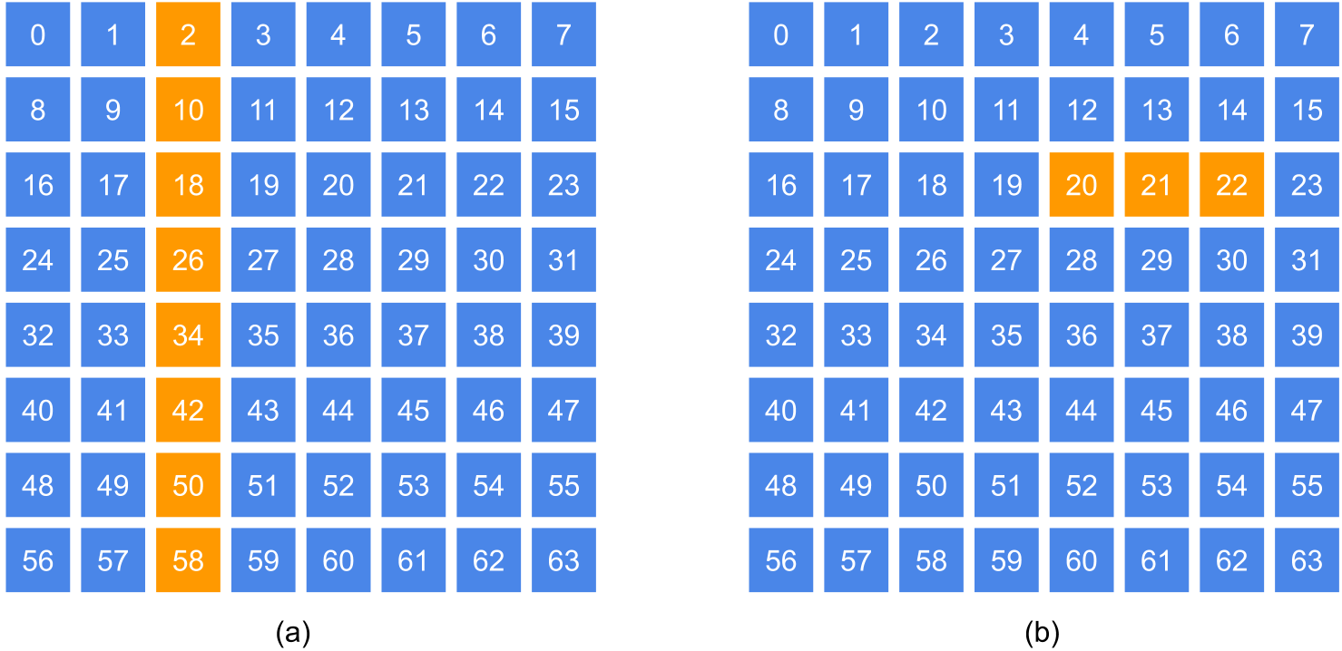
Let’s look at some examples. All are based on an 88 array, initialised explicitly below. The first is shown in Fig. 5.1(a), taking one column of the matrix using both basic and fancy slicing:
# let x = Arr.sequential [|8;8|];;
val x : Owl.Arr.arr =

   C0 C1 C2 C3 C4 C5 C6 C7
R0  0  1  2  3  4  5  6  7
R1  8  9 10 11 12 13 14 15
R2 16 17 18 19 20 21 22 23
R3 24 25 26 27 28 29 30 31
R4 32 33 34 35 36 37 38 39
R5 40 41 42 43 44 45 46 47
R6 48 49 50 51 52 53 54 55
R7 56 57 58 59 60 61 62 63
# Arr.get_slice [ []; [2]  ] x;;
- : Owl.Arr.arr =

   C0
R0  2
R1 10
R2 18
R3 26
R4 34
R5 42
R6 50
R7 58
# Arr.get_fancy [ R[]; I 2 ] x;;
- : Owl.Arr.arr =

   C0
R0  2
R1 10
R2 18
R3 26
R4 34
R5 42
R6 50
R7 58
The second in Fig. 5.1(b) is similar, but retrieves part of a row, again using both methods.
# Arr.get_slice [ [2]; [4; 6] ] x;;
- : Owl.Arr.arr =
   C0 C1 C2
R0 20 21 22
# Arr.get_fancy [ I 2; R [4; 6] ] x;;
- : Owl.Arr.arr =
   C0 C1 C2
R0 20 21 22
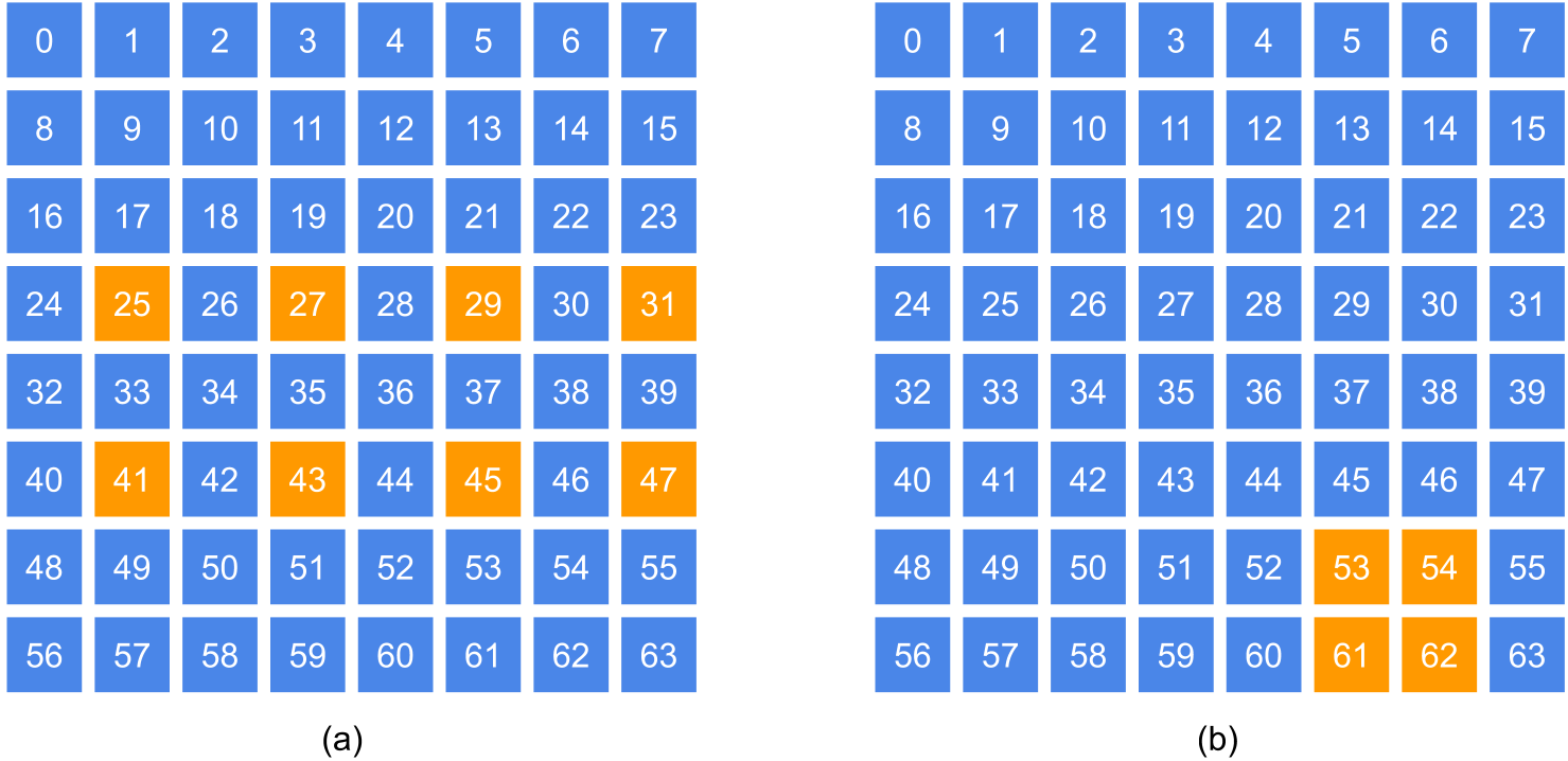
The next example in Fig. 5.2(a) is a bit more complex. It chooses certain rows, and then chooses columns using a fixed step of 2, via fancy slicing:
# Arr.get_fancy [ L [3; 5]; R [1; 7; 2] ] x;;
- : Owl.Arr.arr =
   C0 C1 C2 C3
R0 25 27 29 31
R1 41 43 45 47
Finally, the last example in Fig. 5.2(b) obtains a sub-matrix in a similar manner to examples 1 and 2, using negative integers as indices.
# Arr.get_fancy [ L [-2; -1]; R [-3; -2] ] x;;
- : Owl.Arr.arr =
   C0 C1
R0 53 54
R1 61 62
5.2.3 Advanced Usage
There are more advanced usages of slicing besides what we have just
seen, which we will demonstrate in this section. Based on the same input
matrix x, these examples vary the index s in Mat.get_slice s x. Mat is the
matrix module built on Ndarray; all the following examples also hold for
ndarrays.
[]: take all the elements[ [2]; [] ]: take row 2[ [2] ]: take row 2, but only specify the first dimension[ [1;3] ]: take from row 1 to 3[ [3;1] ]: take from row 3 to 1, same as the example above but in reverse order
Let’s look at some more complicated examples.
[ [1;3]; [3;5] ]take from row 1 to 3 and column 3 to 5, so a sub-matrix ofx[ [1;-1]; [] ]take from row 1 to the last row[ [0;-1;2] ]take the rows with even indices, i.e., 0;2;4;6[ []; [1;-1;2] ]take columns with odd indices, i.e.,1;3;5;7[ [-1;0] ]reverse all the rows of x[ [-1;0]; [-1;0] ]reverse all the elements of x, same as applying reverse function[ [-2]; [0;-1;3] ]take the second last row, at column indices 0, 3, and 6
The following examples show how to use slicing to achieve some even more complicated operations. We use a 55 sequential matrix for illustration.
# let x = Mat.sequential 5 5;;
val x : Owl.Mat.mat =

   C0 C1 C2 C3 C4
R0  0  1  2  3  4
R1  5  6  7  8  9
R2 10 11 12 13 14
R3 15 16 17 18 19
R4 20 21 22 23 24
In the first example, the reverse function treats a matrix as a one-dimensional
vector and reverses its elements. This operation is equivalent to flipping in both
vertical and horizontal directions.
let reverse x = Mat.get_slice [ [-1;0]; [-1;0] ] x;;

# reverse x;;
- : Owl.Arr.arr =

   C0 C1 C2 C3 C4
R0 24 23 22 21 20
R1 19 18 17 16 15
R2 14 13 12 11 10
R3  9  8  7  6  5
R4  4  3  2  1  0
The second function rotates a matrix 90 degrees clockwise. As we can see, slicing leads to very concise code.
let rotate90 x = Mat.(transpose x |> get_slice [ [];[-1;0] ]);;

# rotate90 x;;
- : Owl.Mat.mat =

   C0 C1 C2 C3 C4
R0 20 15 10  5  0
R1 21 16 11  6  1
R2 22 17 12  7  2
R3 23 18 13  8  3
R4 24 19 14  9  4
The last function cshift performs a right circular shift along the columns of a
matrix.
let cshift x n =
  let columns = Mat.col_num x in
  if columns = 0 then Mat.copy x
  else
    let n = ((n mod columns) + columns) mod columns in
    let indices = List.init columns (fun i -> (i - n + columns) mod columns) in
    Mat.get_fancy [R []; L indices] x;;
let _ = cshift x 0;;
Applying this to the previous x should produce the following output:
# cshift x 2;;
- : Owl.Mat.mat =

   C0 C1 C2 C3 C4
R0  3  4  0  1  2
R1  8  9  5  6  7
R2 13 14 10 11 12
R3 18 19 15 16 17
R4 23 24 20 21 22
5.3 Broadcasting
We now introduce the broadcasting operation. In contrast to indexing and slicing which must be explicitly invoked, broadcasting is usually implicitly invoked when certain conditions are met. This often simplifies code but can sometimes make debugging more complicated.
Many binary mathematical operators take two ndarrays as inputs, e.g., add, sub,
etc. In the trivial case, the inputs should have exactly the same shape. However,
we often operate on two ndarrays whose shapes do not match. Implicitly
extending compatible dimensions of either input to a common shape is called
broadcasting.
Broadcasting can save unnecessary memory allocation. For example, assume we have a
1000500 matrix
x that contains 1000 samples each having 500 features. We want to add a bias vector v of
shape 1500
to each feature. As the shapes of x and v do not match, one approach is to tile v so
that it has the same shape as that of x.
let x = Mat.uniform 1000 500;;
let v = Mat.uniform 1 500;;
let u = Mat.tile v [|1000;1|];;
Mat.(x + u);;
The code above works but uses considerable memory for temporary values.
High memory consumption is not desirable, particularly when running on
resource-constrained devices. So we can use broadcasting to add x and v directly,
without using the tile operation. The returned result is of the same shape as
x.
However, the shapes of two inputs cannot be arbitrarily different in broadcasting, but are subject to some constraints. The rule is much simpler than in slicing: given two matrices/ndarrays of the same dimensionality, for each dimension, one of the following two conditions must hold: either both sizes are equal, or one size is 1.
Here are some valid shapes where broadcasting can be applied between x and
y.
  x : [| 2; 1; 3 |]    y : [| 1; 1; 1 |]
  x : [| 2; 1; 3 |]    y : [| 2; 1; 1 |]
  x : [| 2; 1; 3 |]    y : [| 2; 3; 1 |]
  ...
Here are some invalid shapes that violate the constraint above and prevent broadcasting.
  x : [| 2; 1; 3 |]    y : [| 1; 1; 2 |]
  x : [| 2; 1; 3 |]    y : [| 3; 1; 1 |]
  x : [| 2; 1; 3 |]    y : [| 3; 1; 1 |]
  ...
What if y has lower dimensionality than x? E.g., x has the shape [|2;3;4;5|]
whereas y has the shape [|4;5|]. In this case, y’s dimensionality is expanded to the
same number as x’s. Technically, two ndarrays are aligned at their last dimensions.
In other words, this is done by prepending 1s to the shape of y, making
the new shape of y [|1;1;4;5|]. You can try expand by yourself, as shown
below.
# let y = Arr.sequential [|4;5|];;
val y : Owl.Arr.arr =

   C0 C1 C2 C3 C4
R0  0  1  2  3  4
R1  5  6  7  8  9
R2 10 11 12 13 14
R3 15 16 17 18 19
# let y' = Arr.expand y 4;;
val y' : Owl.Arr.arr =

         C0 C1 C2 C3 C4
R[0,0,0]  0  1  2  3  4
R[0,0,1]  5  6  7  8  9
R[0,0,2] 10 11 12 13 14
R[0,0,3] 15 16 17 18 19
# Arr.shape y';;
- : int array = [|1; 1; 4; 5|]
Next we show three broadcasting examples based on matrices, using both illustrations and code, so that you can better understand how the shapes are extended in broadcasting. The first example in Fig. 5.3 is a vector multiplied by a scalar.

let a = Arr.sequential [|1;3|];;
Arr.mul_scalar a 3.;;
The second example in Fig. 5.4 is adding a matrix and a vector.
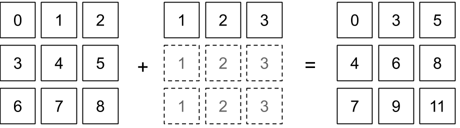
let b0 = Arr.sequential [|3;3|];;
let b1 = Arr.sequential ~a:1. [|1;3|];;
Arr.add b0 b1;;
The third example in Fig. 5.5 is adding a column vector and a row vector.
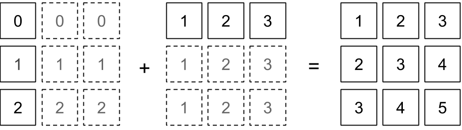
let c0 = Arr.sequential [|3;1|];;
let c1 = Arr.copy b1;;
Arr.add c0 c1;;
The broadcasting operation is transparent so it will be automatically applied if the shapes of two operands do not match and the constraints are met. Operations in Owl that support broadcasting include:
- basic computation:
add,sub,mul,div,pow; - comparison operation:
elt_equal,elt_not_equal,elt_less,elt_greater,elt_less_equal,elt_greater_equal; - other:
min2,max2,atan2,hypot,fmod.
5.4 Tensors
We finish this chapter by briefly introducing the concept of tensor. Many people
use tensor and n-dimensional array interchangeably but there are differences between
them. A tensor can be represented by an array of components in a chosen
basis, but those components must also obey certain transformation rules.
For example, in a three-dimensional vector space we might have a vector
with components [0, 1, 2]. We can find each component using a single
index. This vector is an object in the space, and it stays the same even if we
change the basis. If we do change the basis, its components must be updated
accordingly. In this way we represent tensors as ndarrays, but a stored array alone
does not specify how its components transform. In numerical libraries, the
word tensor is also commonly used simply to mean a multi-dimensional
array.
Consider a single vector with component column in a basis . We can change the basis to via an invertible matrix , with . The component column in the new basis is then , written as:
| (5.1) |
Here . We call these components contravariant because they transform inversely to the basis change. Note that we use superscripts to denote them.
As a comparison, think about a linear functional represented by a row , so that is a scalar. Such functionals form the dual vector space. To keep unchanged under the same basis change, the row must transform as , or in components:
The functional is called a covector, and its components are denoted with subscripts. We can further extend this to matrices. Consider a linear mapping from the vector space to itself, represented by a matrix . With the change of basis, the map remains the same, but its matrix becomes , or:
Again, note that we use both a superscript and a subscript for the linear map , since its components have one contravariant index and one covariant index.
We can further extend this process to tensors with multiple contravariant and covariant indices. A tensor is an object independent of the basis, while its components transform as shown in Eq. 5.2. Here are the contravariant indices and are the covariant indices.
| (5.2) |
One of the important operations on tensors is the tensor contraction, applied to two tensors producing a third tensor through a summation process. Suppose we have tensor and , and you can see that a pair of indices, one covariant of and one contravariant of , are labelled with the same letter . This implies a summation over those two indices. As a result of summation, a new tensor has the indices of the tensors and except for the pair of indices over which the contraction operations took place. In this example, the contraction can be expressed as:
We can compute such contractions using the contract2 function in the
Ndarray module. It takes an array of int * int tuples specifying pairs of
zero-based axes in the two input ndarrays; paired axes must have equal
sizes.
let x = Mat.uniform 3 4;;
let y = Mat.uniform 4 5;;

let z1 = Mat.dot x y;;
let z2 = Arr.contract2 [|(1,0)|] x y;;
Tensor contraction is not limited to matrices. For example, we have two three-dimensional arrays and , and aim to compute the matrix so that:
| (5.3) |
The implementation is similar:
let x = Arr.sequential [|3;4;5|];;
let y = Arr.sequential [|4;3;2|];;
let z1 = Arr.contract2 [|(0, 1); (1, 0)|] x y;;
The pairs mean that axis 0 of x is contracted with axis 1 of y, and axis 1 of x with axis 0 of y.
Here x stores
in the order
and y stores
in the order ,
leaving a result of shape [|5;2|]. We can verify Eq. 5.3 with the naive
contraction summation below, and then check if the two results z1 and z2 are the
same.
let z2 = Arr.zeros [|5;2|];;

let _ =
  for h = 0 to 2 do
    for k = 0 to 3 do
      for i = 0 to 4 do
        for j = 0 to 1 do
          let r = (Arr.get x [|h;k;i|]) *.
            (Arr.get y [|k;h;j|]) in
          Arr.set z2 [|i;j|] ((Arr.get z2 [|i;j|]) +. r)
        done
      done
    done
  done;;
Tensor contraction can also express the convolution operations we will introduce in the signal and neural network chapters.
In brief, convolution is a mathematical way of combining two signals to form a third. Each discrete signal can be represented as a vector, matrix, or ndarray. We will see that convolution is a central operation in convolutional neural networks, and it can be expressed as a series of contraction computations.
As to the implementation, both tensor contraction and discrete convolution can be implemented using general matrix multiplication, or GEMM, a core functionality of BLAS. As we introduced in Chap. 4, GEMM is efficiently implemented in various highly optimised numerical libraries such as OpenBLAS and MKL. To achieve efficiency, tensor contraction implementations can use axis permutations and reshaping to transform contractions into GEMM. Note that using BLAS operations to implement tensor contraction may incur performance and storage overhead. High-performance implementation of the contraction operation has been a research topic in computation related fields [2, 3].
Contraction can also be used to implement other operations that might initially
seem unrelated to matrix multiplication. For example, it can be applied to a single
ndarray to sum along a diagonal using the contract1 function, as the code below
demonstrates.
# let x = Arr.sequential [|2;2;3|];;
val x : Owl.Arr.arr =

       C0 C1 C2
R[0,0]  0  1  2
R[0,1]  3  4  5
R[1,0]  6  7  8
R[1,1]  9 10 11
# let y = Arr.contract1 [|(0,1)|] x;;
val y : Owl.Arr.arr =
  C0 C1 C2
R  9 11 13
Many tensor operations involve summation over particular indices. Therefore in applications such as linear algebra and physics, the Einstein notation is used to simplify expressions [1, Chap. 1, pp. 5–7]. In the mixed-index convention used here, it omits the summation symbol for an index appearing twice in a term, once as a superscript and once as a subscript; no index may occur three times or more in a term. For example, the matrix multiplication notation can be simplified to . The free indices and remain on both sides. Eq. 5.2 can also be greatly simplified in this way.
Tensor calculus is frequently used in physics and engineering, in areas including relativity, quantum physics, and fluid mechanics. More details about tensor calculus are beyond the scope of this book, and we refer readers to work such as Dullemond and Peeters [1] for a deeper understanding of this topic.
5.5 Summary
The -dimensional
array is the most fundamental data type in numerical computing, and we will use it
throughout this book. This chapter explained the details of Owl’s Ndarray module,
including creation, property extraction, manipulation, serialisation, and so on. We
also introduced slicing and broadcasting of ndarrays thoroughly. Mastering these
topics requires practice, and this chapter provides many examples. We finished
this chapter by briefly discussing the difference between a tensor and an
ndarray.
Bibliography
- [1]
- Dullemond K, Peeters K. Introduction to tensor calculus. Lecture
notes; English translation 2008/2010, original Dutch edition 1991.
https://ita.uni-heidelberg.de/~dullemond/lectures/tensor/tensor.pdf. - [2]
- Abdelfattah A, Baboulin M, Dobrev V, Dongarra J, Earl C, Falcou J, Haidar A, Karlin I, Kolev T, Masliah I, Tomov S. High-performance tensor contractions for GPUs. Procedia Computer Science. 2016 Jan 1;80:108-18.
- [3]
- Matthews DA. High-performance tensor contraction without transposition. SIAM Journal on Scientific Computing. 2018;40(1):C1–C24.
- [4]
- Dean J, Ghemawat S. MapReduce: simplified data processing on large clusters. Communications of the ACM. 2008 Jan 1;51(1):107-13