CHAPTER 07
Signal Processing
We rely on signals such as sound and images to convey information. Signal processing is the field concerned with analysing, generating, and transforming signals. Its applications can be found in a wide range of fields: audio processing, speech recognition, image processing, communication systems, data science, etc. In this chapter we focus on Fourier Transform, the fundamental tool in signal processing and modern numerical computing. We introduce its basic idea, and then demonstrate how to perform FFT in OCaml with examples and applications. We also cover the relationship between FFT, convolution, and filters.
For the second edition, the three CSV inputs are reproducible synthetic teaching
data generated by generate_inputs.py. The historical filenames are retained, but
these files contain no measured solar observations, recorded phone call, or real Google
prices.
7.1 Discrete Fourier Transform
We begin with an example. Consider a piece of audio lasting 10 seconds. It can clearly be described in the time domain by plotting its sound pressure against time. On the other hand, perhaps less obviously, it can also be described in the frequency domain. For example, an ideal sinusoidal tone at A#4 has a frequency of about 466.16 Hz in equal temperament with A4 tuned to 440 Hz. Its amplitude, phase and duration are also needed to describe the signal. Of course, real-world sounds such as water flowing or wind whispering are not usually so pure, typically being compounded from different frequencies. How should we describe the frequencies used then?
That’s where the Fourier Transform comes in, starting from a fundamental insight: all signals, whether sound waves or electromagnetic fields, can be described as a waveform, and under suitable conditions, waveforms can be represented by sums or integrals of sinusoids of different frequencies [21]. The Fourier Transform is the tool to break down a signal wave into different sinusoids.
More formally, we can represent a signal with the values of some quantity as a function of time: , or its complex spectrum , which contains amplitude and phase information as a function of frequency. They are two representations of the same thing, and the Fourier Transform converts between them as shown in Eq. 7.1. These two equations show the Fourier transform, and the inverse Fourier transform [2], which changes a signal from the frequency domain back to the time domain.
In computer-based numerical computation, signals are often represented discretely as a finite sequence of sampled data rather than as continuous values, giving rise to the Discrete Fourier Transform (DFT) [3]. Suppose we have represented a signal by a complex vector that contains elements. To get the Fourier Transform vector , the DFT and its inverse are given in Eq. 7.2, where and . and are indices that range from to . 1
What can we do if we know how a sound is composed? Think of a classic example where we need to reduce high-pitched noise in some music. If the noise occupies frequencies that can be separated from the music, we can attenuate those components in the frequency domain and convert the signal back to the time domain using the inverse Fourier transform. Similarly, we can reduce noise in an image by filtering its frequency components before inverting the transform. Filtering can also remove useful detail when signal and noise occupy the same frequencies. We show several such examples in Sec. 7.3.
There are many many more applications of DFT than just de-noising though [4]. We all use Fourier Transform every day without knowing it: mobile phones [5], image and audio compression [6], communication networks [7], large scale numerical physics and engineering [8], etc. In many ways it is the cornerstone of computational mathematics. An important reason for its popularity is that it can be implemented very efficiently as the Fast Fourier Transform.
7.2 Fast Fourier Transform
A problem with the DFT is that if you follow its definition in implementation, the computational complexity of your algorithm is : computing each of the components of in Eq. 7.2 requires multiplications and additions. Therefore naive DFT implementation does not scale well with input size. Fast Fourier Transform (FFT) algorithms reduce this complexity to . An early form is found in work by Gauss dating from around 1805; the publication by James Cooley and John Tukey in 1965 made the approach widely known [9]. In the radix-2 case, with a power of two, the DFT can be split into two sub-DFTs: one consisting of the elements of the signal in the even index positions, and the other consisting of the elements of the signal in odd positions:
The key to enabling this step is the fact that . According to Eq. 7.3, one DFT can be reduced into two DFTs each only half the original length, and then the second half is multiplied by a factor and added to the first half. The half signal can be further halved, and so on and so on. There are logarithmically many recursion levels, with linear work at each level. At the base of this recursion is the fact that a DFT on a single number returns just the number itself. As you can see, this is a typical divide-and-conquer algorithm design.
Detailed mathematical analysis of the Fourier Transform is beyond the scope of this book, and we encourage readers to consult one of the many classic textbooks on this topic such as Phillips et al [10]. We focus here on introducing how to use the FFT implementation and its applications in OCaml code. Hopefully these materials are interesting enough to encourage you to investigate more.
The implementation of the FFT module in the Owl library uses the PocketFFT [11]
C++ backend. The core functions in the FFT module are fft and its inverse ifft,
corresponding to the two equations in Eq. 7.2. Tbl. 7.1 lists the basic functions in
Owl_fft.D, used below. Their inputs are ndarrays. The FFT module provides S and
D submodules for single and double precision, each handling the corresponding real
and complex array types, and a Generic interface. The optional axis selects the
array axis to transform and defaults to the last axis. For irfft, n specifies
the real output length along that axis. With the defaults used here, the
forward transform is unscaled and the inverse is divided by the transform
length.
Owl_fft.D.
| Functions | Description |
fft ~axis x | one-dimensional discrete Fourier Transform |
ifft ~axis x | one-dimensional inverse discrete Fourier Transform |
rfft ~axis x | one-dimensional discrete Fourier Transform for real input |
irfft ~axis ~n x | inverse transform from a half-spectrum to real output |
7.2.1 Example: 1-D Discrete Fourier Transforms
We next show how to use these functions with some simple examples. More complex and interesting ones will follow in the next section.
Let’s start with the most basic fft and its inverse transform function ifft.
First, we create a complex 1-D ndarray that contains 6 elements as input to
fft.
# let a = [|1.;2.;1.;-1.;1.5;1.0|];;
val a : float array = [|1.; 2.; 1.; -1.; 1.5; 1.|]
# let b = Arr.of_array a [|6|]
    |> Dense.Ndarray.Generic.cast_d2z;;
val b : (Complex.t, Bigarray.complex64_elt) Owl.Dense.Ndarray.Generic.t =

       C0      C1      C2       C3        C4      C5
R (1, 0i) (2, 0i) (1, 0i) (-1, 0i) (1.5, 0i) (1, 0i)
We then apply the FFT:
# let c = Owl_fft.D.fft b;;
val c : (Complex.t, Bigarray.complex64_elt) Owl_dense_ndarray_generic.t =

         C0                 C1                 C2        C3                C4                C5
R (5.5, 0i) (2.25, -0.433013i) (-2.75, -1.29904i) (1.5, 0i) (-2.75, 1.29904i) (2.25, 0.433013i)
The input and output of fft are both complex ndarrays. When the
original samples are real, as here, the spectrum has conjugate symmetry:
for
. Its
magnitude is therefore symmetric between positive and negative frequencies; this is
not true for arbitrary complex input. Bin zero is the DC component, followed by
positive-frequency bins and then negative-frequency bins in wrapped order. For even
, bin
is the
Nyquist component. For real input, the nonnegative-frequency half-spectrum is
sufficient for plotting, but reconstruction must also account for its conjugate
half.
# let d = Owl_fft.D.ifft c;;
val d : (Complex.t, Bigarray.complex64_elt) Owl_dense_ndarray_generic.t =

       C0      C1      C2       C3        C4      C5
R (1, 0i) (2, 0i) (1, 0i) (-1, 0i) (1.5, 0i) (1, 0i)
The function ifft takes the frequency domain result c produced by fft and
reconstructs the original time domain signal. Since we do not change the frequencies
generated by fft, the inverse FFT should recover the original input up to
floating-point round-off, as in this example.
But simply manipulating arrays does not make very impressive examples. We next plot the FFT of the sum of two sine waves showing the power of FFT to separate signals of different frequencies. This example uses 600 sampling points and the sample spacing is seconds.
# module G = Dense.Ndarray.Generic;;
module G = Owl.Dense.Ndarray.Generic
# let n = 600.;;
val n : float = 600.
# let t = 1. /. 800.;;
val t : float = 0.00125
# let x = Arr.mul_scalar (Arr.sequential [|int_of_float n|]) t;;
val x : Owl.Arr.arr =

  C0      C1     C2        C597   C598    C599
R  0 0.00125 0.0025 ... 0.74625 0.7475 0.74875
First, we create 600 sample times in seconds, with a step size of 0.00125 seconds; the last sample is at 0.74875 seconds.
# let y1 = Arr.((50. *. 2. *. Owl_const.pi) $* x |> sin);;
val y1 : Owl.Arr.arr =

  C0       C1       C2        C597     C598     C599
R  0 0.382683 0.707107 ... 0.92388 0.707107 0.382683
# let y2 = Arr.(0.5 $* ((80. *. 2. *. Owl_const.pi)
    $* x |> sin));;
val y2 : (float, Bigarray.float64_elt) Owl_dense_ndarray_generic.t =

  C0       C1       C2          C597      C598      C599
R  0 0.293893 0.475528 ... -0.475528 -0.475528 -0.293893
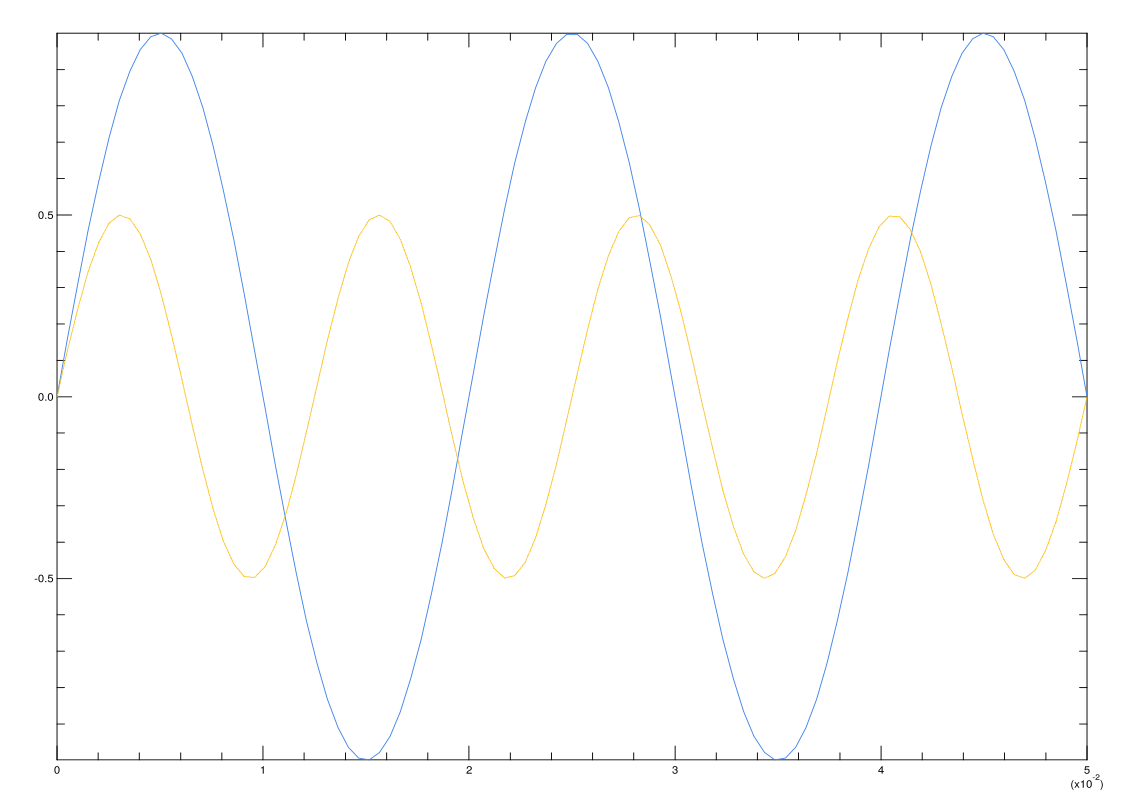
Next we create two sine signals of different frequencies: , , at 50 and 80 Hz respectively, shown in Fig. 7.1a. We then mix them together.
# let y = Arr.(y1 + y2) |> G.cast_d2z;;
val y : (Complex.t, Bigarray.complex64_elt) G.t =

       C0             C1            C2               C597           C598            C599
R (0, 0i) (0.676576, 0i) (1.18264, 0i) ... (0.448351, 0i) (0.231579, 0i) (0.0887908, 0i)
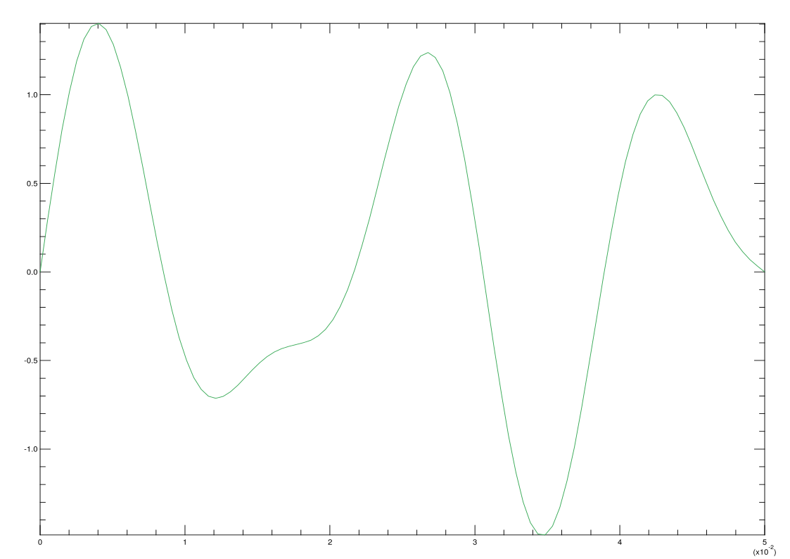
The combined signal in Fig. 7.1b shows an irregular shape. Next, we apply FFT on this mixed signal:
# let yf = Owl_fft.D.fft y;;
val yf : (Complex.t, Bigarray.complex64_elt) Owl_dense_ndarray_generic.t =

             C0                      C1                       C2                         C597                    C598                     C599
R (5.02734, 0i) (5.03096, 8.16436E-14i) (5.04187, -1.90459E-13i) ... (5.06014, -2.24884E-13i) (5.04187, 1.92987E-13i) (5.03096, -8.12175E-14i)
Each complex coefficient represents one frequency bin. We can plot its magnitude,
represented by z in the code below; these are unnormalised FFT magnitudes, not the
amplitudes of the original sinusoids.
# let z = Dense.Ndarray.Z.(abs yf |> re);;
val z : Owl.Dense.Ndarray.Z.cast_arr =

       C0      C1      C2        C597    C598    C599
R 5.02734 5.03096 5.04187 ... 5.06014 5.04187 5.03096
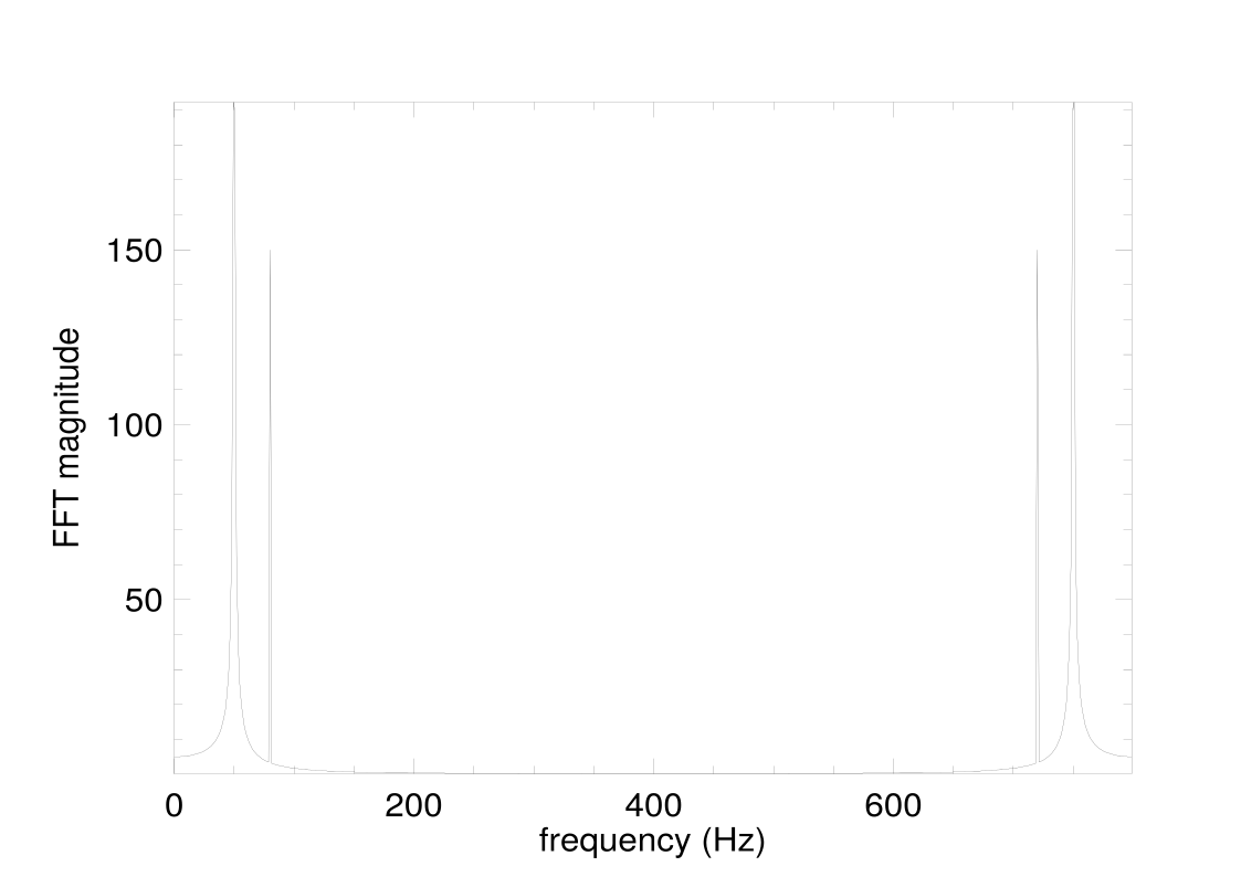
Finally, we plot the result using the code below. The plot is shown in Fig. 7.1c. This plot uses all 600 bins on the axis . Values above 400 Hz represent wrapped negative frequencies: the peaks near 720 and 750 Hz mirror the components at 80 and 50 Hz. The bin spacing is Hz, so 50 Hz lies between bins and its energy spreads into neighbouring bins.
let h = Plot.create "plot_sine_3.pdf" in
let frequency = Arr.mul_scalar (Arr.sequential [|int_of_float n|]) (1. /. (n *. t)) in
Plot.set_xlabel h "frequency (Hz)";
Plot.set_ylabel h "FFT magnitude";
Plot.plot ~h frequency z;
Plot.output h;;
The other two functions, rfft and irfft, handle real-valued signals: rfft
transforms real input into a complex half-spectrum, and irfft reconstructs real
output from that spectrum. Using them can sometimes make code cleaner. For
example, we can apply rfft directly to a real ndarray rather than first casting it to
a complex array, and apply irfft to the result to recover the real input.
The odd-length smoothing example below uses the provided irfft_exact
helper.
7.3 Applications of FFTs
There are numerous applications of the FFT, but we pick three here to demonstrate the power of FFT using OCaml. The first is to find a period in a synthetic sunspot-like series, and the second is about identifying dialled digits from audio. Both are inspired by examples in Moler [12]. The third is about image processing. Together these applications demonstrate the wide usage of FFT in various scenarios.
7.3.1 Finding the Period of Sunspots
On the Sun’s photosphere, sunspots appear as spots darker than the surrounding areas, and their number changes according to a certain cycle. Measured sunspot data are available from SILSO [13]. Here we use a synthetic annual series labelled from 1700 to 2020, with an injected 11-year cycle, varying amplitude and small noise. This provides a reproducible example of period detection; it is not an estimate from observations of the Sun.
let data = Owl_io.read_csv ~sep:';' "sunspot_full.csv";;
let data = Array.map (fun x -> Array.map float_of_string x)
  data |> Mat.of_arrays;;
let x = Mat.get_slice [[];[0]] data;;
let y = Mat.get_slice [[];[1]] data;;
We can visualise the data x (year) and y (synthetic count) as in Fig. 7.2.
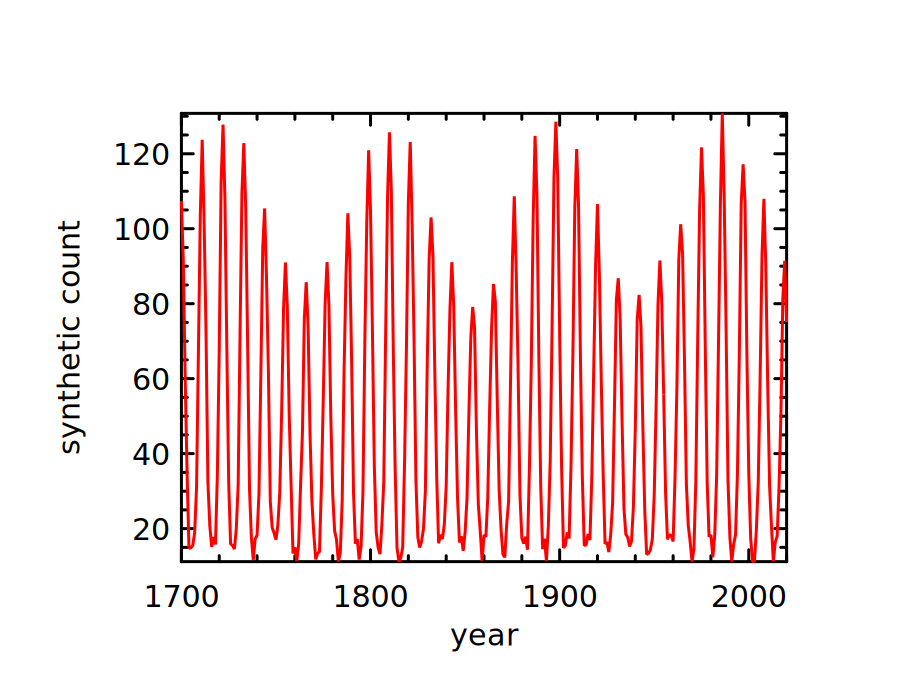
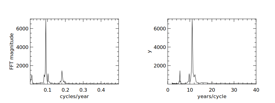
The figure suggests a cycle of about 10 years, but what period does the strongest
spectral peak indicate? Let’s start by applying the FFT to this synthetic signal. This
will show which periodic component is the most prominent. The helper uses rfft and
discards bin zero, which stores the sum of the samples with the default normalisation.
It retains the positive-frequency magnitudes; selecting this half-spectrum does not
halve the frequencies.
let get_frequency y =
  let spectrum = Owl_fft.D.rfft ~axis:0 y in
  let bins = (Dense.Ndarray.Z.shape spectrum).(0) in
  let selected = Dense.Ndarray.Z.get_slice [[1;bins-1];[]] spectrum in
  Dense.Ndarray.Z.(abs selected |> re);;
let get_frequency = get_frequency;;
The frequency (cycle/year) as a unit of measurement seems a bit confusing. To
make the cycle easier to interpret, we also plot the FFT magnitude as a function of
years/cycle. Both are plotted with code below.
let plot_sunspot_freq ~samples p =
  let n = Mat.row_num p in
  let frequency = Mat.of_array
    (Array.init n (fun k -> float_of_int (k+1) /. float_of_int samples)) n 1 in
  let h = Plot.create ~m:1 ~n:2 "plot_sunspot_freq.png" in
  Plot.subplot h 0 0;
  Plot.set_xlabel h "cycles/year";
  Plot.set_ylabel h "FFT magnitude";
  Plot.plot ~h frequency p;
  Plot.subplot h 0 1;
  Plot.set_xlabel h "years/cycle";
  Plot.plot ~h (Mat.scalar_div 1. frequency) p;
  Plot.set_xrange h 0. 40.;
  Plot.output h;;
let p = get_frequency y;;
plot_sunspot_freq ~samples:(Mat.row_num y) p;;
The result is shown in Fig. 7.3. The strongest FFT bin corresponds to about 11.1 years, close to the injected 11-year period. The finite sample length limits the frequency resolution.
7.3.2 Determining the Tone
When we dial a phone number, the sound wave can be seen as a signal. In this
example, we show how to decipher which number is dialled according to the given
soundwave. This example uses a synthesized 11-digit sequence, 12345678901. Each
digit has 5000 tone samples followed by 1000 silent samples, at a sampling rate of
8192 Hz. Let’s first load and visualise them.
let fs = 8192.;;
let data = Owl_io.read_csv ~sep:',' "touchtone.csv";;
let data = Array.map (fun x -> Array.map float_of_string x)
           data |> Mat.of_arrays;;
let data = Mat.div_scalar data 128.;;
The generator specifies a sampling rate (fs) of 8192. We have a segment of
signal that shows a sequence of synthesized touch tones. We can visualise the
signal:
let tone_times = Mat.div_scalar (Mat.sequential 1 (Arr.shape data).(1)) fs;;
The result is shown in the left subfigure of Fig. 7.4. The 11 dense segments correspond to the 11 synthesized digits. We can recover the two frequencies in each segment and check which digit they identify.
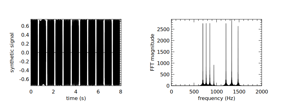
Each touch tone combines two different frequencies: one from a low-frequency group and one from a high-frequency group. The 11 digits in this sequence use seven frequencies from the 12-key keypad shown in Tbl. 7.2. These combinations are specified for dual-tone multi-frequency signalling (DTMF) in ITU-T Recommendation Q.23 [14]. The full scheme also includes a fourth high-frequency column for keys A–D, which this example does not use. Therefore, we can use FFT to decompose the soundwave for each digit into its two basic frequencies, and check this table to find out the answer. Let’s start by applying the FFT to the original data.
let yf = Owl_fft.D.rfft data;;
let y' = Dense.Ndarray.Z.(abs yf |> re);;
let n = (Arr.shape y').(1);;
let x' = Mat.linspace 0. (fs /. 2.) n;;
We plot y’ against x’ similarly using the previous plotting function, and the
result is shown in the right side of Fig. 7.4.
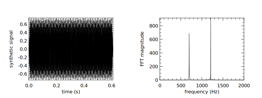
We can use the first tone as an example to find out the two frequencies from which it is composed. Let’s start by getting a subset of the signal:
let data2 = Arr.get_slice [[];[0; 4999]] data;;
We then perform the same process as before producing the results shown in
Fig. 7.5. It shows that the first digit is mainly composed of two frequencies, about
697 and 1209 Hz. Looking them up in Tbl. 7.2, we find that the first digit is
1. You can verify the remaining digits by repeating the same procedure.
7.3.3 Image Processing
FFT remains a powerful tool as the dimensionality of data increases. It can be used for a wide range of image processing tasks such as blurring, compression or denoising. In this section, we demonstrate an image denoising example. The basic idea is similar to the preceding case: an image can be decomposed into two-dimensional spatial frequency components. Here we use a low-pass filter to suppress rapid variations. This can reduce noise, but high spatial frequencies also carry edges and fine detail, so removing them blurs the image; small coefficients do not necessarily represent noise.
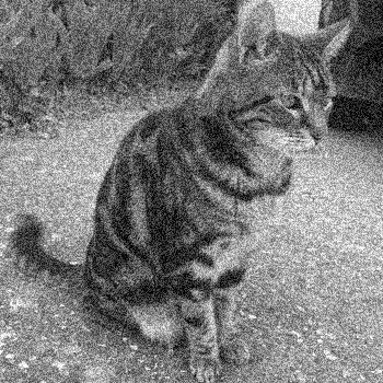
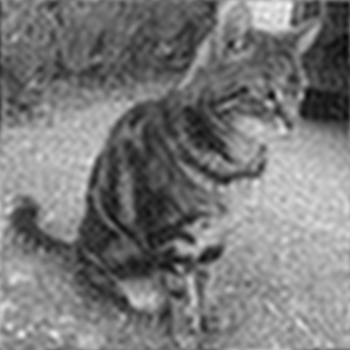
As input, we use a cat image as shown in Fig. 7.6a. As a tool for image
processing in OCaml, we use the imageUtils.ml script which reads images of PPM
format into an ndarray, or saves an ndarray into PPM image. The script is included
in the code repository of this book.
#use "imageUtils.ml";;
module N = Dense.Ndarray.D;;
module C = Dense.Ndarray.Z;;
As a first step we read the image into an ndarray using the function
load_ppm. Since this is a grayscale image, we need only process one single
channel of this array, which is a matrix having all elements in the range 0 to
255.
let img_arr = load_ppm "cat_noise.ppm" |> Dense.Ndarray.Generic.cast_s2d
  |> N.get_slice [[];[];[0]];;
let shp = N.shape img_arr;;
let h, w = shp.(0), shp.(1);;
let img = N.reshape img_arr [|h; w|]
  |> Dense.Ndarray.Generic.cast_d2z;;
The next step is simple: applying the fft2 function on the image matrix.
This function performs a 2-dimensional FFT on the matrix, i.e. it performs
FFT on the input matrix twice, once horizontally, and once vertically. The
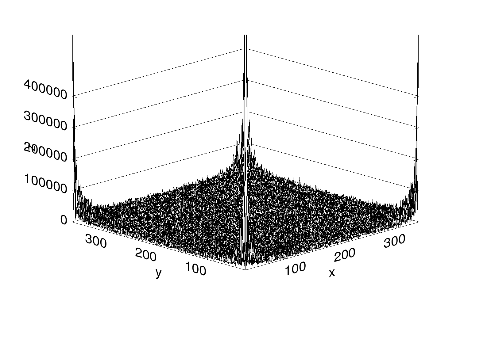
magnitudes of the resulting frequency coefficients can be visualised as in
Fig. 7.7a. This surface contains contributions from both the image and its
noise.
let img_fft = Owl_fft.D.fft2 img;;
visualise_img img_fft "img_fft1.pdf";;
We can apply different kinds of filters on this frequency map img_fft to remove
unwanted frequencies. We choose to use a simple one that keeps only the frequencies
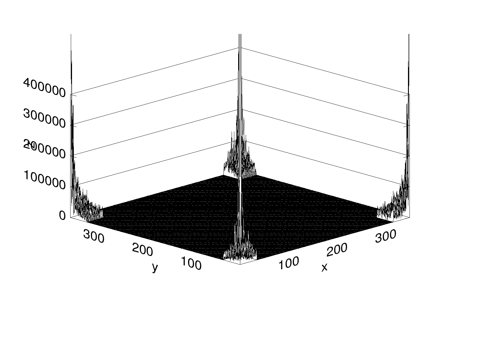
on the four “corners” of this matrix, setting the rest to zero. In the unshifted FFT
layout, these corners contain low spatial frequencies of both signs. We can achieve
this with some slicing techniques.
let sub_length x frac =
  (float_of_int x) *. frac |> int_of_float;;

let h1 = sub_length h 0.1;;
let h2 = sub_length h 0.9;;
let w1 = sub_length w 0.1;;
let w2 = sub_length w 0.9;;
let index_0 = [ R [h1; h2]; R []];;
let index_1 = [ R [0; h1]; R [w1; w2] ];;
let index_2 = [ R [h2; h-1]; R [w1; w2] ];;
let slice_0 = C.get_fancy index_0 img_fft;;
let slice_1 = C.get_fancy index_1 img_fft;;
let slice_2 = C.get_fancy index_2 img_fft;;

let _ = C.set_fancy index_0 img_fft
  (C.shape slice_0 |> C.zeros);;
let _ = C.set_fancy index_1 img_fft
  (C.shape slice_1 |> C.zeros);;
let _ = C.set_fancy index_2 img_fft
  (C.shape slice_2 |> C.zeros);;
visualise_img img_fft "img_fft2.pdf";;
After this process, the frequency map becomes Fig. 7.7b. Finally, let’s apply the reverse 2D FFT on the processed frequency map, and save the result as an image.
let img = Owl_fft.D.ifft2 img_fft |> C.re;;
let image = N.stack ~axis:2 [|img; img; img|];;
let image = N.expand image 4 |> Dense.Ndarray.Generic.cast_d2s;;
let _ = save_ppm_from_arr image "cat_denoise.ppm";;
As shown in Fig. 7.6b, the output has less visible noise and retains the broad features of the cat, but it also loses fine detail and looks blurry.
7.4 Filtering
In Chap. 5, we introduced the generic filter operation, which selects elements
according to a predicate. Signal-processing filters instead modify signal values; the
following examples use weighted combinations of neighbouring samples or frequency
components. A filter is a device or process that removes unwanted components from
a signal. Generally, any system that modifies input signals in certain ways is a filter.
In this section, we introduce how FFT can be applied to perform some filtering tasks
with examples.
7.4.1 Example: Smoothing
Let’s start with smoothing, a common and quite simple filtering task. Suppose we
have a segment of noisy signal shaped like a stock price. In many cases we would like
to remove rapid fluctuations and see a longer-term trend. The second-edition file
goog.csv contains 251 synthetic observations with a slow trend, periodic components
and small noise. It uses the familiar price-table layout for this example; it does not
contain Google quotations. We can load the data into a matrix called “data” using
code below:
let data = Owl_io.read_csv ~sep:',' "goog.csv";;
let data = Array.map (fun x ->
    Array.map float_of_string (Array.sub x 1 6))
    (Array.sub data 1 (Array.length data-1)) |> Mat.of_arrays;;
After removing the sample index, the data contains six numeric columns: synthetic open, high, low, close, adjusted close, and volume. Here we use the synthetic close values in the fourth column of the matrix.
let y = Mat.get_slice [[];[3]] data;;
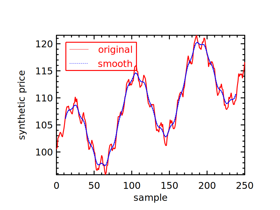
To compute the moving average of this signal, we create a window with 10 elements. For this example, we only use a very simple filter which takes an average of 10 elements.
let filter = Mat.of_array (Array.make 10 0.1 ) 1 10;;
let moving_average_filter = filter;;
We can then slide this filter window along the input signal to smooth the data step by step.
let y' = Mat.mapi (fun i _ ->
    let r = Mat.get_fancy [R [i; i+9]; R []] y in
    Mat.dot filter r |> Mat.sum'
  ) (Mat.get_slice [[0; (Arr.shape y).(0) - 10]; []] y);;
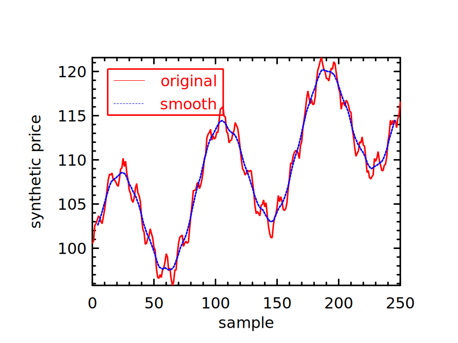
Finally, we plot the resulting smoothed data against the original data. The results are shown in Fig. 7.8. The blue dotted line smooths the jagged original stock price line (red), and represents a smoother view of the synthetic series. Each average is plotted at the centre of its ten-sample window.
7.4.2 Gaussian Filter
The moving average gives equal weight to each element of the window. To change the smoothing profile, we can change this simple filter to another: the Gaussian filter [15]. Instead of giving equal weight to each element in the moving window, the Gaussian filter uses weights proportional to a Gaussian:
| (7.4) |
The code below generates a simple 1-D Gaussian filter and normalises the weights to sum
to one. The window extends to approximately four standard deviations on either side of its
centre. With
sample intervals, radius is 12 and the kernel contains 25 weights.
let gaussian_kernel sigma =
  if not (Float.is_finite sigma && sigma > 0.) then invalid_arg "positive finite sigma";
  let radius = int_of_float (4. *. sigma +. 0.5) in
  let x = Mat.linspace (-.float_of_int radius) (float_of_int radius) (2*radius+1) in
  let kernel = Mat.map (fun a -> exp (-0.5 *. a *. a /. (sigma *. sigma))) x in
  Mat.div_scalar kernel (Mat.sum' kernel);;
let gaussian_kernel = gaussian_kernel;;
let filter = gaussian_kernel 3.;;
Computing the correlation between the filter and input data as before, we get a smoothed curve in Fig. 7.9.
Filters can be described in both the time and frequency domains. In the time domain, the moving-average and Gaussian filters above combine neighbouring samples. In the frequency domain, their frequency responses describe how they change different frequency components. These are complementary descriptions, not mutually exclusive classes. Other designs, such as windowed-sinc and Chebyshev filters, can be chosen for particular frequency-response requirements [16]. There are many types of filters, each with different shape and application scenario, and we cannot fully cover them here. Please refer to some classical textbooks on signal processing such as Smith [17] for more information.
7.4.3 Signal Convolution
So far we have not used FFT functions to perform filtering. In this section we will demonstrate how they can be applied to solve our synthetic price-series smoothing problem. But first, we need to explain the idea of convolution. For discrete signals, it combines two sequences as follows:
| (7.5) |
In Eq. 7.5, and are integer sample indices and operator denotes convolution, and you can think of as a discrete input signal with as the filter. The sliding dot products used above compute cross-correlation. Because the moving-average and Gaussian kernels are symmetric, they also give the corresponding valid convolution values. Computing each convolution output requires summing products over the overlapping samples. Direct computation can become expensive for long signals and kernels; continuous convolution uses an integral instead of this sum.
The FFT can reduce the cost of convolution for sufficiently long inputs and kernels. For finite sequences, multiplication of equal-length DFTs corresponds to circular convolution. To obtain linear convolution, pad both inputs with zeros to a common length of at least , where and are their lengths [17]. With this padding, the convolution theorem gives:
| (7.6) |
To put Eq. 7.6 into plain words: to obtain the DFT of two signals’ convolution, we can simply get the DFT of each signal separately and then multiply them element-wise. That is, convolution in the time domain corresponds to multiplication in the frequency domain. Once you have the , you can simply apply the inverse transform to get .
For the following smoothing example, we specify a filter directly in the frequency domain by retaining low-frequency bins. This is a different filter from the ten-point moving average. Without zero-padding, it treats the finite series as periodic and corresponds to circular convolution with the inverse DFT of the frequency mask. Let’s first move the data to the frequency domain:
let yf = Owl_fft.D.rfft ~axis:0 y;;
The resulting data yf looks like this:
# yf;;
- : (Complex.t, Bigarray.complex64_elt) Owl_dense_ndarray_generic.t =

                        C0
  R0         (27295.2, 0i)
  R1  (-10.0945, 699.605i)
  R2  (-12.0475, 351.714i)
                       ...
R123  (-1.82098, 2.78879i)
R124  (-13.395, -4.45041i)
R125 (-11.4182, -5.74908i)
We keep the first five frequency bins, including the zero-frequency component, setting the rest to zero.
let n = (Dense.Ndarray.Z.shape yf).(0);;
let z = Dense.Ndarray.Z.zeros [|n-5; 1|];;
let _ = Dense.Ndarray.Z.set_slice [[5;n-1];[]] yf z;;
Then, we apply reverse FFT on this processed frequency vector. The book helper
irfft_exact reconstructs the conjugate spectrum and retains the original number of
samples, including an odd length; the current Owl real-inverse entry rejects odd
lengths even when the output length is specified:
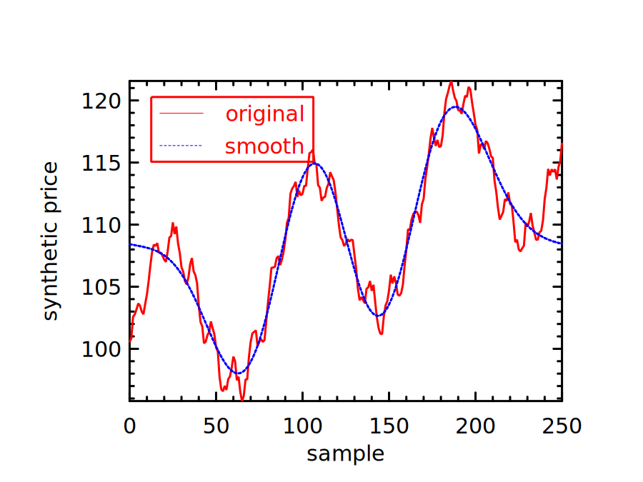
let y2 = irfft_exact ~axis:0 ~n:(Mat.row_num y) yf;;
As with the previous two methods, we can check how the smoothing approach works by plotting the filtered signal. Fig. 7.10 shows the result of retaining only these low frequencies. It is smooth, but is not necessarily a better estimate of the trend: the cutoff determines what is retained, and the periodic assumption can distort the ends of the series.
7.4.4 FFT and Image Convolution
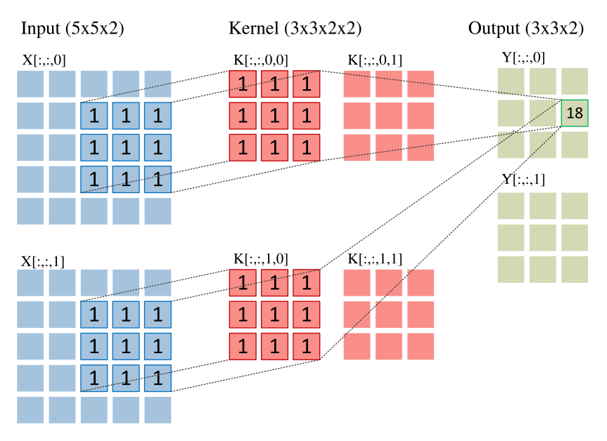
You might have already come across the concept of “convolution” in another context. Indeed, convolution is a core operation in convolutional neural networks (CNNs). In CNNs, it is often applied to multidimensional arrays, but the basic process is similar to what we have described in the previous example. Starting with an ndarray input, another smaller ndarray called “kernel” slides over the input step by step. At each position, an element-wise multiplication and summation are applied, and the result is filled into corresponding position in an output ndarray. This process is illustrated in Fig. 7.11.
Owl has thorough support for convolution operations, including conv1d, conv2d,
and conv3d. The numbers refer to one, two, or three spatial dimensions; the arrays
also have batch and channel axes. Related operations include dilated and transposed
convolutions and the derivatives needed for backpropagation.
It’s totally OK if none of this makes sense to you for now. We will explain the
convolution operations and their usage in neural networks in great detail
in Chapter 11. The point is that the sliding-kernel operation extends to
higher dimensions. Strictly, the neural-network convention used by Owl’s
conv1d is cross-correlation: the kernel is not reversed as it is in mathematical
convolution. For our symmetric moving-average kernel the distinction does not
change the result. We can thus use conv1d to solve the previous smoothing
problem:
let y3 = Arr.reshape y [|1; Mat.row_num y; 1|];;
let f3 = Arr.reshape moving_average_filter [|Arr.numel moving_average_filter;1;1|];;
let y3' = Arr.conv1d ~padding:VALID y3 f3 [|1|];;
If you are interested in checking the result, the vector y3’ contains the data to
plot a smoothed curve. The smoothed data agrees, up to round-off, with that in
Fig. 7.8 since the calculation is essentially the same, albeit obtained with much
less code. We select VALID padding and the original moving-average kernel
explicitly, so that the output agrees with the fully overlapping windows used
above.
FFT is a popular implementation method for convolutions. There has been a lot of research on optimising and comparing its performance with other implementation methods, with practical considerations such as kernel size and implementation details of code [18, 19, 20]. We omit these technical discussions here.
7.5 Summary
This chapter revolves around a fundamental idea in signal processing: the Fourier Transform. We started with its definition, then introduced a crucial idea behind its efficient implementation, namely the Fast Fourier Transform. Owl provides FFT support through its PocketFFT backend. We showed how the FFT functions can be used in OCaml, first with some simple examples, then with three applications: recovering a cycle from a synthetic sunspot-like series, deciphering synthesized dial tones, and de-noising an image. Next, we discussed filtering in signal processing using different techniques, including simple averaging smoothing, Gaussian filtering, and FFT-based filtering. Finally we explained the relationship between the two most crucial computations in numerical applications: FFT and convolution. More about the application of convolution in neural networks will be discussed in Chapter 11 of this book.
Bibliography
- [1]
- McAulay R, Quatieri T. Speech analysis/synthesis based on a sinusoidal representation. IEEE Transactions on Acoustics, Speech, and Signal Processing. 1986 Aug; 34(4):744-54.
- [2]
- Baron Fourier JB. Théorie analytique de la chaleur. Chez Firmin Didot, père et fils; 1822.
- [3]
- Oppenheim AV, Schafer RW, Buck JR. Discrete-time signal processing. 2nd ed. Upper Saddle River: Prentice Hall; 1999.
- [4]
- Bracewell RN. The Fourier transform and its applications. New York: McGraw-Hill; 1986 Feb.
- [5]
- Gupta A. Fourier transform and its application in cell phones. International Journal of Scientific and Research Publications. 2013 Jan; 3(1):1-2.
- [6]
- Strang G. Wavelet transforms versus Fourier transforms. Bulletin of the American Mathematical Society. 1993;28(2):288-305.
- [7]
- Turitsyn SK, Prilepsky JE, Le ST, Wahls S, Frumin LL, Kamalian M, Derevyanko SA. Nonlinear Fourier transform for optical data processing and transmission: advances and perspectives. Optica. 2017 Mar 20;4(3):307-22.
- [8]
- Holberg O. Computational aspects of the choice of operator and sampling interval for numerical differentiation in large-scale simulation of wave phenomena. Geophysical prospecting. 1987 Aug 1;35(6):629-55.
- [9]
- Heideman M, Johnson D, Burrus C. Gauss and the history of the fast Fourier transform. IEEE ASSP Magazine. 1984 Oct;1(4):14-21.
- [10]
- Phillips CL, Parr JM, Riskin EA. Signals, systems, and transforms. 3rd ed. Upper Saddle River: Prentice Hall; 2003.
- [11]
- PocketFFT [Internet]. [cited 2026 Nov 7]. Available from:
https://github.com/mreineck/pocketfft. - [12]
- Moler CB. Numerical computing with MATLAB. Society for Industrial and Applied Mathematics; 2004 Jan 1.
- [13]
- SILSO. Sunspot
Number: data files [Internet]. Royal Observatory of Belgium [cited 2026
Nov 11]. Available from:
https://www.sidc.be/SILSO/datafiles. - [14]
- International Telecommunication Union. Technical
features of push-button telephone sets. Recommendation Q.23; 1988 Nov
25.
https://www.itu.int/rec/T-REC-Q.23-198811-I/en. - [15]
- Blinchikoff HJ, Zverev AI. Filtering in the time and frequency domains. Krieger Publishing Co., Inc.; 1986 Jun 1.
- [16]
- Widmann A, Schröger E, Maess B. Digital filter design for electrophysiological data-a practical approach. Journal of neuroscience methods. 2015 Jul 30;250:34-46.
- [17]
- Smith SW. The scientist and engineer’s guide to digital signal processing. San Diego: California Technical Pub.; 1997 Jan 1.
- [18]
- Fialka O, Cadik M. FFT and convolution performance in image filtering on GPU. InTenth International Conference on Information Visualisation (IV’06) 2006 Jul 5 (pp. 609-614). IEEE.
- [19]
- Kolba D, Parks TW. A prime factor FFT algorithm using high-speed convolution. IEEE Transactions on Acoustics, Speech, and Signal Processing. 1977 Aug;25(4):281-94.
- [20]
- Vasilache N, Johnson J, Mathieu M, Chintala S, Piantino S, LeCun Y. Fast convolutional nets with fbfft: A GPU performance evaluation. arXiv preprint arXiv:1412.7580. 2014 Dec 24.
- [21]
- Oppenheim AV, Willsky AS, Nawab SH. Signals and systems. 2nd ed. Upper Saddle River: Prentice Hall; 1997.